Chapter 15/16: Mapping the ecogeographic distribution of biodiversity and GIS tools for plant germplasm collectors

M. van Zonneveld
Bioversity International, Regional Office for the Americas, Cali, Colombia
E-mail: m.vanzonneveld(at)cgiar.org
E. Thomas
Bioversity International, Regional Office for the Americas, Cali, Colombia
E-mail: e.thomas(at)cgiar.org
G. Galluzzi
Bioversity International, Regional Office for the Americas, Cali, Colombia
E-mail: g.galluzzi(at)cgiar.org
X. Scheldeman
Bioversity International, Regional Office for the Americas, Cali, Colombia
E-mail: xschelde(at)gmail.com

	Chapter15/16 - 2011 version (0.7 MB)	Chapter 15 - 1995 version (0.5 MB)	Chapter 16 - 1995 version (0.2 MB)
	Open the full chapter in PDF format by clicking on the icon above.

This chapter is a synthesis of new knowledge, procedures, best practices and references for collecting plant diversity since the publication of the 1995 volume Collecting Plant Diversity; Technical Guidelines, edited by Luigi Guarino, V. Ramanatha Rao and Robert Reid, and published by CAB International on behalf of the International Plant Genetic Resources Institute (IPGRI) (now Bioversity International), the Food and Agriculture Organization of the United Nations (FAO), the World Conservation Union (IUCN) and the United Nations Environment Programme (UNEP). The original text for chapter 15: Mapping the Ecogeographic Distribution of Biodiversity and chapter 16:Geographic Information Systems and Remote Sensing for Plant Germplasm Collectors (both authored by L. Guarino) has been made available online courtesy of CABI. The 2011 update of the Technical Guidelines, edited by L. Guarino, V. Ramanatha Rao and E. Goldberg, has been made available courtesy of Bioversity International.

Please send any comments on this chapter using the Comments feature at the bottom of this page. If you wish to contribute new content or references on the subject please do so here.

Back to list of chapters on collecting

References for this chapter

Internet resources for this chapter

 

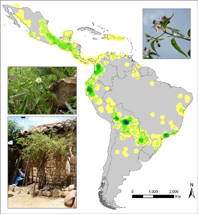
	Observed richness of wild Capsicum species. (Cover photos from left-below to the right: C. eximium Hunz., C. baccatum L., C. eximium fruits and flower. Map and photos: M. van Zonneveld. Data source: Georeferenced specimen and genebank passport data made available by herbaria and genebanks through the Global Biodiversity Information Facility.)

Abstract

Ecogeographic studies provide critical information on plant genetic resources (PGR) to assess their current conservation status and prioritize areas for conservation. They have also proven useful for effective genebank management, such as the definition of core collections and identification of collection gaps. Geographic information systems (GIS) are useful tools for mapping ecogeographic distributions of biodiversity. GIS allow complex analyses to be performed, as well as clearly visualizing results in maps, which facilitates decision making and implementation of conservation policies by authorities.

Technological advances in both software and hardware, together with the increased availability and accessibility of geographical, environmental and biodiversity data through the internet, have led to increased application of GIS analyses for conservation and use of PGR in the last two decades. In this update, we give an overview of relevant techniques and advances in ecogeographic studies of PGR to analyse biodiversity data based on collected data and to target further collection. We commence with providing some general recommendations that are important when setting up new research projects that are aimed at assessing the conservation status of PGR and/or monitoring trends in (agricultural) biodiversity on the basis of ecogeographic data.

A brief introduction of commonly used methods and techniques for the analysis of inter- and intraspecific diversity is provided, including multivariate methods such as clustering and ordination. We also elaborate mapping of (agricultural) biodiversity data and emphasize the importance of ensuring good data quality. Furthermore, we provide a synopsis of available methods for distribution modelling and present an overview of useful open-access and commercial statistical and GIS packages. We conclude our update with an identification of future challenges and research needs.

 

Introduction

Ecogeographic studies refer to the process of collecting, characterizing, systemizing and analysing different kinds of data pertaining to target taxa within a defined region (Maxted et al. 1995). These kinds of studies are important for the formulation and implementation of more targeted and, hence, more effective conservation strategies for plant genetic resources (PGR) (Guarino et al. 2005). Taxonomic, morphological and genetic data can provide critical information about the diversity present in specific geographic areas, which, in turn, can be used for various purposes, such as the assessment of the current conservation status of PGR and to prioritize areas for in situ conservation. At the ex situ level, combining climate and other ecological information of an accession’s collection site – from its passport data – with corresponding morphological or molecular characterization data has also proven useful for effective genebank management (e.g., definition of core collections, identification of collection gaps, etc.). Geographic information systems (GIS) are useful tools for this type of analysis (Guarino et al. 2002). GIS tools allow complex analyses to be done, as well as visualizing results in clear maps, which facilitates decision making by relevant authorities and encourages the development and implementation of conservation policies (Jarvis et al. 2010). GIS analysis is carried out on the basis of coordinate systems; hence, the importance of georeferenced biodiversity data in ecogeographic studies.

The analytical approaches presented in chapters 15 and 16 of the 1995 edition of the Technical Guidelines are still valid. However, since 1995, technological advances and the growing availability of computers and portable global positioning system (GPS) receivers have led to the increased application of GIS analyses at various levels (including spatial data collected by rural communities and forest dwellers). The number and power of statistical programmes have also become much more advanced, especially with respect to analysis of genetic diversity (Holderegger et al. 2010). Furthermore, the general accessibility and use of the internet has created a leap forward in the sharing of geographical, environmental and biodiversity data. One of the notable examples is the Global Biodiversity Information Facility (GBIF) (www.gbif.org), a platform providing public access to biodiversity data from national museums, herbaria and genebanks worldwide. In October 2010, the GBIF contained roughly 39 million georeferenced plant observations.

 

Current status

Preliminary data handling

The following three paragraphs present several key recommendations on how to initiate an ecogeographic survey for PGR, following Guarino et al. (2005). Any such study should start with a commission statement that clearly states the objectives and the methodological design, including a sound strategy for data collection. Taxonomical experts should be identified who can provide key information about the target taxa and validate the results/products obtained from ecogeographic analyses and research, such as distribution maps and the results of collection gap analysis (Ramirez-Villegas et al. 2010). When available, it can be extremely useful to involve networks of taxonomical experts in such studies. Experts from the Latin American Forest Genetic Resources Network (LAFORGEN) have, for example, provided basic information about reproductive behaviour (breeding systems, pollination and seed dispersal systems) of prioritized tree species in the MAPFORGEN project (www.mapforgen.org).

Given the continuous changes in taxonomical classification of plants (APG III 2009), it is of utmost importance to determine upfront the taxonomical boundaries and nomenclature that will be used. The online database of the US Germplasm Resources Information Network (GRIN) (www.ars-grin.gov/cgi-bin/npgs/html/index.pl) provides a useful reference in this respect. All the same, it is strongly advisable to consult other databases such as the Plant List (www.theplantlist.org) or the International Plant Names Index (IPNI) (www.ipni.org) as well as to refer to other data sources such as experts, monographs and Floras.

The geographical extent and boundaries of the target region depend on the objectives of the study. For example, a study focused on assessing the status of PGR for strengthening national conservation programmes will be limited to the country’s national territory. In most other cases, since the occurrence of cultivated and wild taxa does not follow political boundaries, the target region of ecogeographic studies will be defined based on available knowledge about the distribution and diversity of taxa, compiled from literature reviews (e.g., Zeven and De Wet 1982) and consultation with experts from national or international agricultural research centres.

Data collection

Before starting actual collection of field data, preparation of a clear list of descriptors for passport data is recommended. In order for data from different studies and sources to be comparable, data collection, compilation and management require standardization. Data standards for multicrop descriptors have been developed to standardize passport data, morphological characterization and evaluation. These standards make the resulting information comparable across germplasm samples (Alercia et al. 2001). In a similar manner, in order to enable comparison of molecular characterization of crop species, minimum standard sets of markers have been suggested (Van Damme et al. 2010).

Original fieldnotes should be saved carefully and adequately backed up to allow for cross-checking of data at a later stage. A backup should also be made of the original data files stored in a notebook or GPS receiver. Field data can be integrated with additional data retrieved from online portals with data from genebanks and herbaria, contributing to more comprehensive analyses on the distribution and conservation of PGR (see table 15/16.1 for an overview).

Table 15/16.1: Online PGR Documentation Systems and Portals for Sharing Biodiversity Data

Portal	Data type	Website
Germplasm Resources Information Network (GRIN), National Plant Germplasm System (NPGS)	Passport, characterization and taxonomic information of PGR conserved by the United States Department of Agriculture (USDA)	www.ars-grin.gov/npgs/index.html
System-wide Information Network for Genetic Resources (SINGER)	Passport data of the PGR conserved by the Consultative Group on International Agricultural Research (CGIAR) Centres	http://singer.cgiar.org
EURISCO	Access to all ex situ PGR information in Europe.	http://eurisco.ecpgr.org
Genesys	Passport, characterization and evaluation data for the 22 most important crops, from CGIAR Centres, EURISCO and GRIN	www.genesys-pgr.org
Global Biodiversity Information Facility (GBIF)	Passport data from herbaria and genebanks from all around the world	www.gbif.org
SpeciesLink	Passport data from the Brazilian herbarium information system	http://splink.cria.org.br/index?&setlang=en
JSTOR Plant Sciences	Taxonomic information and historic herbarium samples	www.plants.jstor.org
Botanical Research and Herbarium Management System (BRAHMS)	Instructions for mapping species distribution summaries and diversity indices	http://dps.plants.ox.ac.uk/bol

 

Recording geographical data is normally done directly in the field by assigning geographical coordinates through the use of a GPS receiver. The geographic coordinate system in GPS receivers can usually be adjusted according to the user’s preferences. Two commonly used systems are longitude/latitude and Universal Transverse Mercator (UTM). Longitude/latitude is preferred in large-scale studies, such as for taxa that occur across different countries. The longitude/latitude coordinate system in combination with the World Geodetic System (WGS) 1984 is recommended in the data standards for multicrop descriptors (Alercia et al. 2001) and is the coordinate system of many freely available spatial datasets (see table 15/16.2 for an overview), which makes it the preferred option in combination with WGS 1984 for easily combining different spatial datasets. For studies at lower administrative units (e.g., province, department, state), the UTM may be preferred because of the low distortion at this scale and the ease in calculating geographic distances. To be able to carry out GIS analysis with the collected data, longitude/latitude coordinates should be in decimal degrees. If longitude/latitude coordinates of collection sites have been listed in degrees, minutes and seconds, a special formula can be applied to convert these coordinates into decimal degrees (see chapter 2 of Scheldeman and van Zonneveld 2010) .

Table 15/16.2: Some Spatial Data Sources and Tools

Climate

Interpolated climate surfaces for the globe up to 1km resolution: WorldClim (www.worldclim.org) Downscaled layers from future climate models (GCMs): Climate Change Agriculture and Food Security (CCAFS) (www.ccafs-climate.org) Reconstructed paleoclimates: US National Oceanic and Atmospheric Administration (NOAA) (www.ncdc.noaa.gov/paleo/paleo.html)

Topography

Elevation, watershed and related variables for the globe at 1km resolution: US Geological Survey (USGS) (http://eros.usgs.gov) High-quality elevation data for large portions of the tropics and other areas of the developing world: SRTM 90m Elevation Data (http://srtm.csi.cgiar.org)

Remote sensing (satellite)

Various land-cover datasets: Global Land Cover Facility (GLCF) (http://glcf.umiacs.umd.edu/data) Various atmospheric and land products from the MODIS instrument: National Aeronautics and Space Administration (NASA) (http://modis.gsfc.nasa.gov/data)

Soils

Harmonized World Soil Database (www.iiasa.ac.at/Research/LUC/External-World-soil-database/HTML)

Other spatial data

Relevant links and data at DIVA-GIS website (country level, global level, global climate, species occurrence); near global 90-meter resolution elevation data, high-resolution satellite images (LandSat) (www.diva-gis.org/Data) Spatial database of the world's administrative areas (or administrative boundaries): Global Administrative Areas (GADM) (www.gadm.org) Database with eight million place names with geographical coordinates: GeoNames (www.geonames.org) Automatic georeferencing tools: BioGeomancer (www.biogeomancer.org)

 

Since various identification codes may be used in the different steps of collecting, characterizing and evaluating germplasm material (e.g., collector code, field code, collection code), it is essential to clearly define a unique identification code to be applied to each accession throughout the entire study. This will ensure consistent and unequivocal correspondence between each accession and the complexity of its passport, characterization and evaluation data. It is key to getting confident georeferenced taxonomic, phenotypic or genetic diversity data for ecogeographic studies. The addition of new codes should be considered carefully because more codes may lead to confusion and increase the likelihood of making errors in the documentation system, thus affecting the reliability of the data and reducing the possibility of effectively conserving and using collected and characterized germplasm.

Diversity analyses

Ecogeographic studies related to the conservation and use of PGR are mostly focused at the species or gene level of plant diversity. At the species level, the observed unit of alpha diversity is the species, measured mostly as present or absent in a certain location (species richness). Other parameters of species diversity are evenness and abundance (Magurran 1988). Studies at the gene level can be either interspecific (e.g., phylogenetic studies within a gene pool or clade) and/or intraspecific (i.e., to understand genetic variation between plant individuals of the same species or within and between populations of plant species). For the purpose of measuring genetic variation, the chosen units of diversity may be phenotypic traits (the products of a gene or its expression) or, more directly, variation in sequences of neutral or functional portions of DNA or RNA, measured with the assistance of molecular markers (e.g., SSRs, SNPs, DArT, AFLPs; see De Vicente and Fulton [2004] for an overview of different types of molecular markers).

Richness in species or in the number of alternating DNA sequences in specific parts of a plant species genome (e.g., allelic richness) are straightforward measures of diversity and are commonly used for prioritizing conservation areas of either plant communities – based on number and uniqueness of observed species (Gotelli and Colwell 2001) – or within-species populations identified through molecular markers (Frankel et al. 1995a; Petit et al. 1998). However, richness is sensitive to sample bias – the situation where an uneven number of observations or collections has been made across the sampling units included in an ecogeographic study (some units will contain more observations than others). The rarefaction methodology allows correcting such sample bias by recalculating richness on the basis of an equal, user-defined number of observations per sampling unit (Gotelli and Colwell 2001; Petit et al. 1998).

In studies of genetic diversity based on molecular markers, the number of locally common alleles is an important indicator for prioritizing populations of wild and domesticated plant species for in situ conservation. These alleles occur in relatively high frequency over a limited area and can indicate local adaptation to specific environments (Frankel et al. 1995a). Locally common alleles can be identified by statistical programmes for genetic data such as GenAlEx (see table 15/16.3), which identifies alleles with a frequency higher than 5% in a local population and occurring in less than 25% of all populations as locally common alleles (Peakall and Smouse 2006). Another way to detect locally common alleles is with the help of GIS, by identifying those alleles that occur at relatively high frequencies within a given maximum distance (see chapter 5 of Scheldeman and van Zonneveld 2010).

Distance parameters

In diversity analysis, ecological and genetic distances are statistics of central importance that allow investigating the existence of structure and patterns in biodiversity data (beta diversity). This, in turn, is essential for prioritization strategies for in situ conservation (Gallo et al. 2009; Petit et al. 1998; van Zonneveld et al. in prep.), as well as for germplasm management and use, such as in the establishment of core and reserve collections (Frankel et al. 1995b). Ecological distances can be used to calculate how divergent different sampling units are, based on their species or varietal composition, whereas genetic distances are typically used to calculate how divergent within-species individuals or populations are, based on morphological trait or allelic composition. Genetic distances can also be used in phylogenetic studies to order species. Multivariate techniques such as clustering and ordination allow the ordering of units of diversity, such as sampling units, species, plant individuals (within species), on the basis of the ecological or genetic distances between them. Several open-access analysis packages can be useful for carrying out diversity analysis, including the calculation of distance parameters, clustering and/or ordination analyses. Some commonly used programmes for ecological and genetic diversity and structure analysis are listed in table 15/16.3. Additional software for specific genetic analyses is listed in Appendix A of Lowe et al. (2004) and in Excoffier and Heckel (2006).

There is a wide variety of different distance statistics that can be employed, each with different properties. Some distance measures, such as Euclidean distance, are used for calculating both ecological and genetic distances, whereas other measures are generally used for either one of them. Other popular ecological distances include Bray-Curtis, Kulczynski, Hellinger and Chi-square distances (Kindt and Coe 2005). Since the distance measure is the input for subsequent multivariate techniques (e.g., clustering, ordination) and will thus affect the results of this type of analyses, it is important to select an appropriate distance statistic  from the start. A desirable characteristic of any ecological distance parameter is that it assigns the same maximum distance to all pairs of sites that do not share any species (e.g., a property of the Bray-Curtis and Kulczynski distances [Kindt and Coe 2005]). For other features of different ecological distance parameters and how to test them, refer to Kindt and Coe (2005).

Table 15/16.3: Open-Access Applications for Biodiversity and Genetic Analysis

Software	Properties and applications	Source
Biodiversity. R	A single software environment for performing nearly all types of biodiversity analysis; Operates in statistical programme R	Kindt and Coe 2005 http://cran.r-project.org
Vegan	Ordination methods, diversity analysis and other functions for community and vegetation ecologists; Operates in statistical programme R	Kindt and Coe 2005 http://cran.r-project.org/web/packages/vegan/vignettes/intro-vegan.pdf
Biodiversity-Pro	Alpha and beta diversity analysis, multivariate statistics	McAleece et al. 1997 http://gcmd.nasa.gov/records/NHML_Biopro.html
EcoSim	Null model analysis in community ecology	Gotelli and Entsminger 2004 http://garyentsminger.com/ecosim/index.htm
PAST	Developed for paleontology, but offering vast possibilities for (multivariate) biodiversity analysis	Hammer et al. 2001 http://folk.uio.no/ohammer/past
GenStat Discovery	Free version of statistical programme GenStat	www.vsni.co.uk/software/genstat-discovery
Adegenet	Population genetics, including clustering based on Bayesian Information criterion, Discriminant Analysis of Principal Components and spatial Principal Components Analysis; Operates in statistical programme R	Jombart 2008 http://adegenet.r-forge.r-project.org
Structure	Free software package for using multi-locus genotype data to investigate population structure.	Pritchard et al. 2000 http://pritch.bsd.uchicago.edu/structure.html
GenAlEx	User-friendly cross-platform package for population genetic analysis Runs within Excel	Peakall and Smouse 2006 www.anu.edu.au/BoZo/GenAlEx

 

The choice of genetic distance measures largely depends on the type of data (phenotypic, or dominant or co-dominant molecular marker data) and whether distance is calculated between individuals or between groups of individuals. A guide to which measures of genetic distances may be most appropriate for different situations is provided by Lowe et al. (2004) and De Vicente et al. (2004b). Popular genetic distance parameters include Nei’s standard genetic distance, the Arc distance or the Manhattan distance for quantifying distances between populations, and the Tanimoto or Jaccard distance for quantifying distances between individuals (Geburek and Turok 2005).

A series of distance parameters can be used when estimating the variation in phenotypic traits between individuals of the same species. This applies to data analyses from so-called “common garden” experiments (e.g., Willemen et al. 2007). In such experiments, plant material collected in different sites is established in field trials under a common environment, in order to reduce the variance by the environmental effect in the expression of phenotypic traits. When a dataset contains both nominal and continuous morphological data, the Gower distance can be used (Grum and Atieno 2007; Willemen et al. 2007). The Ward-MLM distance (Franco et al. 2010) is useful for combining phenotypic and molecular marker data in clustering or ordination. In light of the different properties of the different genetic distance statistics, it is important to note that care must be taken when comparing different studies that use different distance parameters (Finkeldey 2005).

Distance measures can also be used to test the hypothesis that individuals located further away from each other are also genetically more distant. To do this, Mantel correlation is often used to calculate between pair-wise geographical and genetic distances. Mantel tests can be carried out in packages like Adegenet or GenAlEx (see table 15/16.3). Other types of distances can be compared with genetic distances through Mantel tests as well, such as environmental distances, like climate or soil, to examine whether individuals from different ecological zones are also genetically more distinct (Kozak et al. 2008). In GIS programmes, environmental data (climate, topography, soils) for each collection site can be easily extracted from freely available spatial data maps and exported to a spreadsheet for further statistical analysis (Scheldeman and van Zonneveld 2010). Table 15/16.2 provides an overview of important sources and tools for spatial data.

Clustering

Clustering refers to methods that draw on the distance parameters discussed above for assigning units of diversity such as sampling units, species, within-species individuals or populations, into groups or clusters whose members show a certain level of similarity for measured characteristics. Many hierarchical and non-hierarchical clustering methods exist and it is practically impossible to choose a “best” method because of their heuristic nature. The value of clustering is limited because the outcomes can change substantially depending on different combinations of distance parameters and clustering methods. Therefore, this type of analysis is useful for exploring variation within collected data, but it should not be considered as definitive proof of clear patterns in data (Kindt and Coe 2005). Whereas a markedly discontinuous structure in data will likely be detected by almost any method, a more gradual or continuous structure will be more difficult to detect by cluster analyses (Jongman et al. 1995) and ordination methods are in these cases more appropriate than clustering methods (Kindt and Coe 2005). It is possible to evaluate the clustering performance of a distance statistic by calculating the cophenetic correlation, which compares the distances between observation points calculated by a given distance parameter with the corresponding distances between these points in the cluster diagram (for further information see Kindt and Coe [2005]).

Grum and Atieno (2007) provide a user-friendly introduction to clustering with continuous and nominal variables in the free statistical programme R. A frequently used programme to assign plant individuals to genetic clusters on the basis of molecular markers is Structure (Pritchard et al. 2000), which uses a Bayesian approach to determine the probabilities of plant individuals belonging to each cluster from a predefined number of clusters. Evanno et al. (2005) present a method to determine, within the Structure environment, the number of clusters that best describe the genetic structure of the gene pool. These clusters can also be geographically visualized in GIS (Vigouroux et al. 2008).

Ordination

The basic aim of ordination is to represent observations (e.g., different species across a climate gradient, or allelic composition of within-species plant individuals) and sampling units (e.g., different plots in which species composition is determined, or sample tissues from different individuals that are used for determining allelic composition) in a two-dimensional space in such a way that points that are close together are more similar than points that are further apart. Ordination allows simultaneous representation of observations and sampling units on the same plane. Observations of species or plant individuals (within a species) that are plotted close together have a higher likelihood to occur in sampling units with more similar characteristics (e.g., because they share the same environmental niche or morphological or molecular characteristics) as compared to points that are plotted further apart. Likewise, points representing sampling units that are close together correspond to sampling units that are similar in species, morphological trait or allelic composition, whereas points that are far apart correspond to samples that are dissimilar in this respect. This combined visualization allows one to relate patterns in observations with underlying patterns in the relative sampling units (for instance, between-species similarity and similarity between the plots where these species were observed).

Two general approaches are used in ordination. In direct (or constrained) gradient analysis, direct relationships are sought between (1) the occurrence and/or abundance of species, varieties or alleles and (2) specifically measured (environmental) variables that characterize the sampling units in which these species, varieties or alleles were observed. Observations and sampling units are arranged in a virtual space along axes that are linear combinations of these explanatory variables (e.g., environmental variables), and the predictive power of each of the respective variables is determined (Höft et al. 1999). By contrast, indirect (or unconstrained) gradient analysis focuses entirely on observations and allows maximum explanation of variation without the restriction of explanatory variables (Jongman et al. 1995). This type of analysis is particularly useful when there is no clear foreknowledge about variables that might explain variation between the observations.

Most types of direct and indirect gradient analysis can be divided into two main types of ordination techniques: those that are related to (1) a linear (monotonic) response model in which the abundance of any observational unit (such as species or within-species plant individuals) either increases or decreases with the value of each of the explanatory variables (e.g., Principal Components Analysis [PCA] and Redundancy Analysis [RDA]) and (2) a unimodal response model, where any observational unit occurs within a limited range of the explanatory variables (e.g., Correspondence Analysis [CA] and Canonical Correspondence Analysis [CCA]) (Jongman et al. 1995). Given that the unimodal distribution is more common in nature than a linear distribution, it might be more advantageous to use unimodal over linear response models (Kindt and Coe 2005). According to Jongman et al. (1995), it is advisable to start analyzing biodiversity data by using unimodal models (CA, Detrended Correspondence Analysis [DCA] or CCA) and to decide afterwards whether one could simplify the model to a monotonic one. Non-metric multidimensional scaling (NMDS) is an additional method for indirect gradient analysis that differs in various ways from nearly all other ordination techniques. It can handle non-linear species responses of any shape and allows the use of any distance parameter (Holland 2008). Table 15/16.4 provides a summary of the different options of ordination techniques.

Table 15/16.4: Ordination Techniques

	Unconstrained or indirect gradient analysis	Constrained or direct gradient analysis	Distance measure
Unimodal response model	Correspondence Analysis (CA)	Canonical Correspondence Analysis (CCA)	Chi-square distance
	Detrended Correspondence Analysis (DCA)	Detrended Canonical Correspondence Analysis (DCCA)	Chi-square distance
Monotonic or linear response model	Principal Components Analysis (PCA)	Redundancy Analysis (RDA)	Euclidean distance
	Principal Coordinates Analysis (PCoA) = metric multidimensional scaling	Distance-based Redundancy Analysis (db-RDA) Canonical Analysis of Principal Coordinates (CAP)	Any distance
Non-linear response of any shape	Non-metric multidimensional scaling		Any distance

 

Mapping ecogeographic data

Data quality control

In mapping the ecogeographic distribution of the target taxa, it is crucial for the data to be of high quality and precise (i.e., to contain a minimum number of errors at a specified scale of study). Therefore it is very important to check the quality of the data before they are used in analysis. During field collection, it is recommended that detailed passport information be noted down in a field book and that this original information be carefully saved to enable any error that might emerge during data analyses to be tracked back. Chapman (2005a,b) and chapter 4 of Scheldeman and van Zonneveld (2010) explain several ways to check the quality of georeferenced data, including verification of consistency between the data on (1) the administrative unit (country, provinces, departments) mentioned in the passport data of a collection or observational record as it was registered in the field and (2) the administrative unit in which it is mapped in a GIS programme.

Another way to identify potentially erroneous points is to carry out an outlier analysis, which identifies georeferenced records of the target taxa that are located in atypical climates compared to the climatic niche in which records of the taxa normally occur (Scheldeman and van Zonneveld 2010). Such records can be erroneous due to incorrect coordinates or taxonomic misidentification. However, they might also effectively represent individuals at the marginal ends of a taxon’s distribution range, which could contain valuable traits for adaptation to atypical site conditions. Yet another possibility is that areas with a distinct climate, where outliers are located, have been undersampled in comparison to other areas. If this is the case, these areas could be considered for further collection. For these reasons, when possible, it is recommended that the field book containing original passport information of a record in an atypical climate be consulted (or contact the collector in case the data came from a third party) to find out whether the record is an error. If the outlier appears not to be an error, it can be useful to further evaluate the properties of the plant individuals located in the outlier location based on molecular or phenotypic characterization. If plant individuals possess properties of human interest, it can be worth considering further exploration of the surrounding areas for other plant individuals/populations with similarly interesting traits.

One should also bear in mind that in many cases, data originating from herbaria and genebanks (e.g., freely available from GBIF) were not generated for the purpose of biogeographic studies, and they are often the result of ad hoc collecting or non-systematic and uneven sampling efforts (Chapman 2005a). Frequently, specimens/accessions have been collected mostly or exclusively from areas that are easily accessible or where a taxon is known to occur, thus negatively affecting the representativeness of the data (Hijmans et al. 2000). Such sample bias can later be corrected – although only to a certain extent – with methods such as rarefaction and distribution modelling (see Scheldeman and van Zonneveld [2010] for further details). The best way to prevent sample bias is, of course, by establishing a sound strategy for data collection, although it should be acknowledged that this is not always possible.

Georeferencing

Georeferencing, which assigns geographical coordinates to collection records or observation data missing such coordinates, can substantially increase the number of sound observation records of the target taxa and consequently improve the quality of ecogeographic studies. Specimen label data from collections such as herbaria, which do not include geographical coordinates but do include precise information about the locality where the specimen was collected or observed, can be georeferenced using either gazetteers that can be downloaded from the DIVA-GIS website (see table 15/16.2) or automated online gazetteers such as GeoNames (www.geonames.org) and BioGeomancer (www.biogeomancer.org). Google Earth can be useful for georeferencing records as well, especially those that are taken at a specific distance along the road between two localities. BioGeomancer provides a significant step towards automated georeferencing: it currently encompasses natural language processing (geo-parsing) to interpret the descriptive locality text, place-name lookup to register localities with known geographic coordinates, and ambiguity analysis to self-document uncertainties in resulting geographic descriptions. At the time of this publication, work was still in progress for a workbench that will allow georeferencing of batches of data, speeding up the handling of large bodies of observation records.

Plant diversity, distribution and conservation

The number and frequency of species, varieties or alleles in distinct sampling units within a study area (alpha diversity) are the principal subjects of the spatial analysis of diversity to prioritize areas for conservation in situ and collection of PGR. Sampling units may refer to previously identified sites, administrative units or grid cells of any chosen size. In many cases, such as the example in chapter 15 of the 1995 edition of the Technical Guidelines, species distribution is mapped on the basis of observed species presence in the cells of a grid that covers the study area. At a national or continental level, this grid size may be as large as 50 x 50 km, as used in the Atlas Florae Europaeae (2011), or 100 x 100 km (about one degree) (Scheldeman et al. 2007). In this respect chapter 5 of Scheldeman and van Zonneveld (2010) provides working examples to practice mapping species and allelic richness in grid cells with a point to grid analysis in DIVA-GIS.

The advantage of using grid cells is that these allow the comparison of diversity between sampling units of similar geographical size throughout the extent of the study area. DIVA-GIS and other GIS programmes –among those reviewed in Steiniger and Bocher (2008) – can be used to carry out grid-based diversity analysis (see table 15/16.5 for open-access and commercial packages) and have been applied in several studies to assess the distribution and conservation status of crop gene pools (e.g., Hijmans and Spooner 2001; Jarvis et al. 2003; Scheldeman et al. 2007). Other ways to map distribution and richness are by means of circular area (Hijmans and Spooner 2001) or circular neighbourhood (Hijmans et al. 2005b; Scheldeman and van Zonneveld 2010).

Methods have been developed to optimize the number of conservation areas based on the number of species, varieties or alleles in different units and how they complement each other. DIVA-GIS also includes a reserve selection algorithm, developed by Rebelo and Siegfried (1992), which calculates the minimum number of areas (grid cells) necessary to conserve a given number of species, varieties or alleles of the gene pool under study (Hijmans et al. 2001). It ranks grid cells that should be given priority for conservation in the following order: first priority is given to the grid cell with the highest alpha diversity; subsequent priority is given to those grid cells that best complement the initial ones because they contain the highest number of new species, varieties or alleles that were not found in the previously selected grid cells (beta diversity). Chapter five of Scheldeman and van Zonneveld (2010) explains how to carry out such a reserve selection.

Distribution modelling

For most plant species, including many crop wild relatives and socioeconomically important tree species, only a limited amount of information on their natural distribution is currently available (Nic Lughadha et al. 2005). Distribution modelling or ecological niche modelling is considered a useful tool for overcoming the lack of concrete information on the natural distribution of species (Guarino et al. 2002; Hernandez et al. 2006). It aims to distinguish between zones where the species could potentially occur (i.e., areas with similar environmental conditions to the defined ecological niche) and areas where the species is likely to be absent because the local environment is different from the ecological niche. Distribution models can thus be used to predict the full natural distribution ranges for plant species on the basis of records of presence and absence by defining the ecological niche of a species on the basis of statistical (empirical) relations between occurrence and environmental factors. GIS are very useful in this respect because they allow extraction of information from environmental data layers relative to sites where a species has been observed, as well as to sites where it is known to be absent, and allows visualizing and editing the outcomes of the model on a map. Environmental data layers in distribution modelling can be derived from datasets like those listed in table 15/16.2. Depending on the modelling programme used, they can consist of only continuous variables, such as climate data derived from WorldClim (Hijmans et al. 2005a), or also include nominal variables, such as maps of vegetation or soil type. While distribution modelling is traditionally used to predict the distribution of species, it can also be applied for intraspecific units of diversity, such as ecotypes or clusters defined on the basis of morphological or molecular markers.
The collection of absence records is a challenge because the reasons for absence are not always clear; it might either be due to ecological characteristics, human disturbance or simply because species presence was overlooked during an inventory or collection. Therefore, distribution modelling often uses presence records only (Pearce and Boyce 2006). Presence records can be derived from herbarium specimens, genebank accessions or vegetation/plant species inventories, which have become increasingly available online through portals such as GBIF (see table 15/16.1).

In addition to understanding the full distribution range of a species, distribution models have also been used in gap analyses to prioritize areas for germplasm collection (Jarvis et al. 2005; Scheldeman et al. 2007). In this respect, a gap refers to a location where a distribution model predicts the potential occurrence of a target taxon, but where specimens and/or germplasm of the taxon have not actually been collected. Ramirez-Villegas et al. (2010) present a method based on the identification of sampling, geographic and environmental gaps to prioritize among taxa. Chapter 6 of Scheldeman and van Zonneveld (2010) explains how to carry out a gap analysis with the use of the distribution modelling programmes Maxent and DIVA-GIS. An important source of guidance is the GapAnalysis portal (http://gisweb.ciat.cgiar.org/GapAnalysis) with its methods for crops and crop wild relatives.

 Table 15/16.5: GIS Packages

Open-source desktop GIS	Properties	Source
DIVA-GIS	Biodiversity analysis, species distribution mapping, etc. Also provides free spatial data for the whole world	www.diva-gis.org
GRASS (Geographic Resources Analysis Support System)	Analysis and scientific visualization, cartography, simulation	http://grass.itc.it/intro
QGIS (Quantum GIS)	Viewing, GRASS-Graphical User Interface	http://qgis.org
uDig (User-friendly Desktop Internet GIS)	Viewing, editing, analysis	http://udig.refractions.net
SAGA (System for Automated Geoscientific Analyses)	Analysis, modelling, scientific visualization	www.saga-gis.org
ILWIS (Integrated Land and Water Information System)	Analysis, integrating image, vector and thematic data	www.itc.nl/Pub/Home/Research/Research_output/ILWIS_-_Remote_Sensing_and_GIS_software.html
OpenJUMP 2002/03	Editing, analysis JUMP Family (Java Unified Mapping Platform)	www.openjump.org
Commercial GIS	Properties	Source
Esri	Products include ArcView 3.x, ArcGIS, ArcSDE, ArcIMS, ArcWeb services and ArcGIS Server.	www.esri.com
Autodesk	Products include Map 3D, Topobase, MapGuide and other products that interface with its flagship AutoCAD software package	http://students.autodesk.com/?nd=download_center&c_key=31305F5F416D657269636173&
Bentley Systems	Include Bentley Map, Bentley Map View and other products that interface with its flagship MicroStation software package	www.bentley.com/en-US/Products/Bentley+Map
ERDAS IMAGINE	Products by ERDAS Inc, include ERDAS ER Mapper, ERDAS ECW JPEG2000 SDK	www.erdas.com/products/ERDASIMAGINE/ERDASIMAGINE/Details.aspx
Intergraph	Products include G/Technology, GeoMedia, GeoMedia Professional, GeoMedia WebMap, and add-on products for industry sectors, as well as photogrammetry	www.intergraph.com
MapInfo	Products by Pitney Bowes, include MapInfo Professional and MapXtreme	www.pbinsight.com/welcome/ten-five/index3.php
Smallworld and Spatial Eye	Purchased by General Electric and used primarily by public utilities	http://site.ge-energy.com/prod_serv/products/gis_software_2010/en/index.htm www.spatial-eye.com/Engels/Spatial-Workshop-features/Direct-access-to-data-in-smallworld-GIS/page.aspx/49

 

Another application of distribution modelling is to examine the impact of climate change on the distribution of plant species of interest and socioeconomic importance, such as crop wild relatives (Jarvis et al. 2008) or timber tree species (Saénz-Romero et al. 2006;van Zonneveld et al. 2009a).

It is important to note that distribution modelling can be used to better understand species distribution and to help prioritize areas for germplasm collection only when some information about a species is already available. There is no standard in terms of the minimum number of observation points required, as this will often relate to the nature of the species: for rare species or species with a restricted niche, only a small number of presence records may be sufficient, while for species with a broad niche and extensive distribution range, a higher total number of records is desirable. Although it is difficult to provide strict guidelines on the minimum number of presence records necessary for credible distribution modelling, a number of illustrative examples exist:

• Scheldeman et al. (2007) used a minimum of 10 points for rare Vasconcellea species with a known restricted distribution.

• The MAPFORGEN project (MAPFORGEN 2011), which evaluates the natural distribution of 100 species native to Latin America, used a minimum number of 20 species presence records.

• van Zonneveld et al. (2009b) worked with a minimum number of 50 presence records for two pine species with a broad geographic distribution range throughout Southeast Asia.

Modelling a species’ natural distribution is done under several conditions, the most important being (1) the species should be in a state of equilibrium with its environment (in other words, the environmental ranges are restricted by competition and predation and not by dispersion limitations) and (2) the available environmental variables (e.g., climate variables) used in the modelling are determinant a-biotic factors in shaping the natural distribution of the species. In practice, one or both of these conditions are often not met; nonetheless, distribution modelling is still a useful tool for approximating the natural distribution of a species and, as such, is relevant for prioritizing conservation activities.

Because the model outcomes are an approximation of the species’ real distribution, it remains a challenge to estimate how representative modelled distributions are. Moreover, the outcomes of distribution modelling can vary depending on the modelling program used, quality of presence records and included environmental layers. The outcomes of these models, although potentially useful, should therefore be validated carefully for in situ conservation planning and targeted collection (Loiselle et al. 2003). There is extensive literature about methods for validating models (e.g., Araújo et al. 2005; Beauvais et al. 2006). DIVA-GIS includes an option to calculate two frequently used indicators of model evaluation – maximum Kappa and Area Under Curve (AUC) of Receiver Operation Curve (ROC) – from cross-validating modelled distribution maps with a subset of the presence records (Hijmans et al. 2005b). Maxent also provides an option to calculate AUC (Phillips 2009), albeit it is argued that other indicators are more appropriate to measure model performance (see Lobo et al. 2008).

Over the years, a wide variety of ecological distribution models have been described in the literature, an exhaustive description of which is beyond the scope of this chapter. In the following section, we give a brief overview of the most popular empirical distribution models that are based on observed data and which assume an equilibrium state of the ecosystem, partly based on Peters (2008).

• Linear Regression models: Regression analysis aims at predicting the pattern in one response variable from the pattern of one or several independent or predictor variables (Kindt and Coe 2005).

• General linear models (GLMs): General linear models were developed for situations when certain aspects of the linear regression model are not appropriate. GLMs provide ways of realistically estimating a function of the mean response (the so-called link function) as a linear combination of a given set of predictor variables (Dobson 2002; Nelder and Wedderburn 1972). Popular GLM models are the Poisson GLM with a logarithmic link function (when data are counts) and the binomial GLM with logit link function (for presence-absence data) (Kindt and Coe 2005).

• General additive model (GAM): The general additive model extends the GLM by fitting nonparametric smoothing functions to estimate relationships between the response and the predictive variables (Hastie and Tibshirani 1986). The smoothing function generates a curve that can flow more freely between the data than a straight line.

• Tree-based techniques: Tree-based techniques partition the predictor (environmental) space into parts and then fit a simple model to each part. Classification (categorical response) and regression (continuous response) trees (CART) (Breiman et al. 1984) are a popular technique. Other methods, such as rule-based classification (Lenihan and Neilson 1993) and maximum likelihood classification (Franklin and Wilson 1991), have been developed. Random Forests is a related technique that differs from ordinary tree-based techniques in that it generates an ensemble of trees instead of a single best tree (Breiman 2001).

• Bayesian techniques: Distribution models based on Bayes’ theorem modify an initial (a priori) estimate of the probability of encountering a species or vegetation type in the landscape by using (1) known preferences (e.g., based on expert knowledge or the literature) of the species or vegetation type for environmental characteristics and (2) information concerning the distribution of these characteristics in the landscape (Guisan and Zimmerman 2000; Tucker et al 1997). However, the quality of the a priori information largely determines the model’s performance.

As mentioned above, this list of techniques is not exhaustive; many others exist, including artificial neural networks (Lek and Guegan 1999), support vector machines (Cortes and Vapnik 1995), the environmental envelope (Busby 1991) and maximum entropy (Elith et al. 2011; Phillips et al. 2006) models.

In terms of software packages, Maxent, which implements a maximum entropy modelling approach, has performed very well in comparison to others (Elith et al. 2006; Hernandez et al. 2006). It has been used to evaluate the outcomes of species distribution models under different sets of environmental layers (Blach-Overgaard et al. 2010) and to compare the outcomes of species distribution model with the use of different presence record datasets (Feely and Silman 2011). Integrated into DIVA-GIS are other two distribution modelling programmes: BIOCLIM and DOMAIN (Carpenter et al. 1993; Hijmans et al. 2005b). Although their statistical algorithms are easier to understand than the one used by Maxent, they have not performed as well in comparative studies (Elith et al. 2006; Hernandez et al. 2006). An advantage of Maxent and Domain is that they allow the inclusion of both continuous variables, such as climate data, and categorical variables, such as layers of vegetation and soil types; BIOCLIM only allows the inclusion of continuous variables. Table 15/16.6 lists some software packages that are commonly used for distribution modelling.

Table 15/16.6: Distribution Modelling Packages

Software	Properties and applications	Source
Maxent	Maximum-entropy approach for distribution modelling	www.cs.princeton.edu/~schapire/maxent
BIOMOD	Ensemble forecasting of species distributions, enabling the treatment of a range of methodological uncertainties and the examination of species-environment relationships	http://r-forge.r-project.org/projects/biomod/
OpenModeller	Cross-platform environment where a fundamental niche modelling experiment can be carried out A number of algorithms are provided as plug-ins, including GARP, Climate Space Model, Bioclimatic Envelopes, Support Vector Machines and others	http://openmodeller.sourceforge.net/
Biomapper	A kit of GIS and statistical tools designed to build distribution models and maps for any kind of animal or plant Centred on the Ecological Niche Factor Analysis (ENFA), which does not require absence data	www2.unil.ch/biomapper/what_is_biomapper.html
DOMAIN	Can operate effectively using only records and a limited number of biophysical attributes	Carpenter et al. 1993
Random Forests	(See text above)	www.stat.berkeley.edu/~breiman/RandomForests/cc_home.htm
GARP	The Genetic Algorithm for Rule-set Prediction (GARP) is a distribution modelling method	Stockwell and Peters 1999

 

Genetic structure and genecological zonation

Spatial patterns of genetic structure are traditionally visualized on spatial data maps by means of vector point data in different colours (e.g., Motamayor et al. 2008) and in pie charts (Trognitz et al. 2011). Pie charts are also used to display similarities and differences in the composition of chloroplast or mitochondrial DNA of different populations (Pautasso 2009). More recently, grid-based analyses based on molecular marker data have been used to develop accurate conservation strategies for PGR (Kiambi et al. 2008; van Zonneveld et al. in prep.) and to understand the origin and domestication of crops (van Etten and Hijmans 2010).

For most tree species and crop wild relatives, information concerning patterns of intra-specific diversity across their distributions, which can help in prioritizing areas for in situ conservation and germplasm collection, is not yet available. In such cases, genecological zonation can provide guidance with respect to the establishment of networks of conservation stands (Graudal et al. 1995). Following the assumption that ecogeographic variation shapes genetic patterns (Byers 2005; Ramanatha Rao and Hodgkin 2002), information about climatic and ecological parameters and topographic barriers can be used to define genecological zones, which putatively correspond to differences between species populations that are likely to be genetically distinct because of limited gene flow and/or local adaptation to specific environmental conditions. To identify different climate zones, for instance, DIVA-GIS can be used to map climate zones on the basis of the WorldClim dataset with the use of the clustering option (Hijmans et al. 2005b). Topographic barriers can be visualized with GIS and used to assign records to different populations separated by mountain ranges or water division lines (see table 15/16.2). Such theoretically constructed zones should ideally be validated by empirical data (ground-truth) in order to allow adjustment or refinement. When genetic (molecular or phenotypic) data exist, clustering or ordination techniques can be used to evaluate how much of the genetic structure can be explained by grouping plant individuals in populations according to genecological zones (e.g., Zhang et al. 2006).

Ecogeographic distribution data of specific taxa can provide measures of their plasticity and adaptation and can be a useful complement to morphological and molecular marker studies (or even serve as proxy if morphological or molecular data are not available). In this context, ecogeographic studies support the prioritization of material to be secured in genebanks (Parra-Quijano et al. 2011) and the establishment of core collections for breeding purposes. A programme like Powercore allows the inclusion of ecogeographic variables, such as climate (continuous) and watersheds (nominal), to calculate a subset that is assumed to be representative for a specific taxon in the complete collection (Kim et al. 2007). Ecogeographic studies are also used for carrying out gap analyses, and the higher the level of spatial coverage, the greater the amount of genetic variation that is likely to be captured. In recent years, methodologies and approaches for assessing gaps in genebank collections and prioritizing taxa to be searched in collection missions have been developed. Maxted et al. (2008) provide a gap analysis based on a combination of taxonomic, genetic and ecogeographic diversity.

When specific accessions from a genebank collection have shown interesting traits in evaluation trials (such as drought tolerance or pest and disease resistance), it can be worthwhile to evaluate genebank accessions collected in the same ecological zone since they will most likely have adapted to a similar environment and might express similar interesting traits. This approach, called Focused Identification of Germplasm Strategy (FIGS) has been used, for example, to pre-select 1320 accessions from a wheat collection of about 16,000, to screen on resistance to powdery mildew. Sixteen percent of the selected accessions showed resistance to the disease (Bhullar et al. 2009).

Monitoring trends in biodiversity

Information about species distribution can be used as an indicator to assess the conservation status of the natural populations of particular plant species. It can be anticipated that species with a narrow and/or fragmented natural distribution are more vulnerable to threats such as changes in land use and climate than species with an extensive and continuous distribution. The World Conservation Union (IUCN) has developed several Red List parameters that are based on species distribution, most notably, the extent of occurrence and area of occupancy (IUCN B criterion). In combination with criteria about observed or expected trends in population size, these parameters provide information about the conservation status of species (IUCN 2008). The distribution-based Red List parameters can be calculated with freely available GIS tools (Willis et al. 2003). In combination with information from species experts, they can be used to evaluate the conservation status of wild species, including crop wild relatives (e.g., VMABCC and Bioversity International 2009).

It is generally accepted that the modernization of agriculture and changes in land use could have a negative effect on the diversity of crop species and their wild relatives (agricultural biodiversity) conserved on farms and at a landscape level, and might lead to genetic erosion at the level of either crop, variety or allele (van de Wouw et al. 2010). Nevertheless, exact, well-quantified measures and evidence of genetic erosion as a consequence of agricultural modernization are scarce. Indeed, under certain conditions, crop diversity might even increase when modern varieties are introduced (Bioversity International 2009). Therefore, it is important to establish adequate indicators and to identify areas where agricultural biodiversity can be monitored. Genetic erosion of crops in specific study areas can be measured by comparing current in situ diversity with the diversity of genebank material collected from the same area in the past (De Haan et al. 2009). The existing genetic diversity can be compared between different types of land use, such as commercial agriculture vs. traditional farming to understand the dynamics in the use of crop diversity (van Heerwaarden et al. 2009). GIS are a useful tool to overlay areas of high crop diversity with thematic maps that provide information about accessibility, ethnicity and land use, among other variables, and to better understand which social and economic variables drive the dynamics in the use of crop diversity (e.g., Willemen et al. 2007)

In terms of indicators, those developed within the IUCN criteria may not be appropriate for monitoring the dynamics in the use of crop diversity since they are limited to monitoring at the species level (rather than intra-specific level). An indicator proposed by the Conference of the Parties to the Convention on Biological Diversity (www.cbd.int) is the total number and share of main crop varieties, but this might not adequately reflect relative changes in crop diversity (Eaton et al. 2006). From a scientific point of view, allelic evenness and richness measured through molecular markers are more appropriate for detecting changes in crop diversity (Eaton et al. 2006). Although molecular marker studies have become increasingly common and can be applied to monitoring trends in agricultural biodiversity, other, non-molecular-based indicators are also recommended (OECD 2003). These include the share of land devoted to non-intensive production/high biodiversity (with varieties specific to such production systems), percentage of seed of three major crops/varieties originating on-farm and number of traditional (low-production) varieties stored in a genebank (Eaton et al. 2006). The monitoring of crop diversity on the basis of commercial and traditional varieties might be particularly relevant for specific crops when a sound inventory of registered varieties is in place (Eaton et al. 2006) or when taxonomic keys to distinguish between crop varieties are defined and accepted, such as in the global project of native maize (Proyecto global de maíces nativos, www.biodiversidad.gob.mx/genes/proyectoMaices.html). However, registration of varieties according to morphological characterization may still lead to a substantial degree of misidentification (van de Wouw et al. 2011; Vigouroux et al. 2008). Since the results for molecular markers are more consistent, standardized sets of these markers (Van Damme et al. 2010) are recommended as indicators in monitoring crop diversity (van de Wouw et al. 2010). For molecular marker studies, young shoots or other vegetative material from individual plants can be collected in the field and simply stored in bags (such as Ziploc® bags) with silica gel before they are sent to a laboratory for molecular analysis.

The disadvantage of molecular markers is that in many cases, neutral diversity is measured within a sampling unit and not, directly, the diversity of genetic resources (i.e., genetic material of current and future use). Although it can be anticipated that in areas with high neutral diversity, there is also a higher likelihood of finding a high diversity of genetic resources, it is worthwhile to include indicators that directly measure the diversity in traits of interest as well (e.g., morphological descriptors, functional molecular markers). Similarly, taxonomic identification remains important. Since this is the basis for limiting the gene pool under study and is essential for identifying target taxa during field collection, it should be combined with monitoring based on molecular markers.

Implementation of the International Treaty on Plant Genetic Resources for Food and Agriculture (www.planttreaty.org) by a growing number of countries calls for increased impetus in developing an integrated, effective, efficient, global approach to conserving PGR for food and agriculture as part of a rational global system. Molecular and other types of indicators for analysing agricultural biodiversity (like those described above) are crucial for improving the extent to which variation can be determined in existing ex situ collections or under on-farm conditions. They can become a powerful tool for planning new and cost-effective collecting missions (Ramanatha Rao and Hodgkin 2002).

 

Future challenges/needs/gaps

Regardless of the advances achieved in the two last decades, further improvements in tools and methodologies for data gathering, quality control, availability and analysis are still called for. Among the needs and gaps whose solution would significantly speed up or improve the quality of research, a few are presented as follows (the list does not pretend to be exhaustive but only to touch upon some challenging areas of improvement).

Increased application of standardized molecular markers as indicators of diversity

The use of standardized sets of molecular markers, as already mentioned, is becoming increasingly necessary in order to allow comparability among the growing body of data on molecular diversity being generated worldwide, at least for major crops. Standardized sets, which basically perform as descriptor lists at the morphological level, already exist, such as the Generation Challenge Programme SSR kits for 11 crops (among which are wheat, rice, maize, potato, sorghum, chickpea, bean) (http://s2.generationcp.org/gcp-tmm/web). Particularly if and when the application of molecular markers becomes standardized, public databases for characterization data should be created and made easily accessible to users, complementing and completing the information on species distribution data found in databases such as GBIF and Genesys (see table 15/16.1). The combined information can indicate hotspots of intra-specific diversity, directing collection missions aimed at material carrying specific traits, informing in situ conservation strategies as well as sampling strategies for detailed monitoring of crop diversity.

Increased use of multi-site evaluations for evaluating environment and climate effects on crop performance

Multi-site trials repeated over a number of growth cycles with crops or varieties grown at different locations allow a cross-comparison of how different environmental and climatic conditions affect the performance of specific accessions that were collected in the past and are being conserved ex situ. The repeated recording of performance data from multi-site trials gives consistency to the predictive power of productivity models and allows improved calibration of the models, themselves, by providing a real-world test of the performance of crops or varieties under different environmental and climatic scenarios. Information about performance will be especially important for understanding how crops and trees can be expected to perform in specific areas under climate change (i.e., under warmer conditions in combination with wetter or drier conditions). Several studies on the impact of climate change on crop performance have been carried out based on field trial data (Lobell et al. 2011; Ortiz et al. 2008). Based on such experiments, promising germplasm adapted to specific environments can be identified.

Availability and integration of additional high-resolution non-climate environmental data in distribution models

One of the challenges of distribution modelling resides in the common assumption that climate is the main variable for species survival, resilience and reproduction. Such an assumption is sometimes problematic (Currie 2001; Turner et al. 2003) and may limit the reliability of the model’s predictions. Although there is consensus that temperature and precipitation are the most important factors determining species distributions, other variables, such as soil properties and radiation, are often crucial as well (Austin 2007).

Specifically, questions are often raised about the lack of consideration of soil variables in models. Although the reliability, accuracy and scale of worldwide soil data are currently not yet as great as the climate variables, quite comprehensive databases, such as the Harmonized World Soil Database (www.iiasa.ac.at/Research/LUC/External-World-soil-database/HTML), exist and could be more consistently integrated into modelling exercises. Initiatives are underway to develop high-resolution soil maps (Sanchez et al. 2009).

Improved integration of additional tools for statistics and data analyses in GIS

Although GIS packages are being constantly improved, and spatial diversity and distribution analysis software (including DIVA-GIS) now includes a good range of statistical tools, further integration of more  advanced and specific statistical power could be envisaged. For instance, the integration of distribution models and R statistics (including the more specific Biodiversity.R package) into GIS would significantly speed up and automate statistical elaborations, saving on the time needed to develop a separate dataset out of the GIS. Additional efforts could be made to incorporate the analyses carried out in genetic statistical programmes (e.g., Adegenet, GenAlEx and STRUCTURE) into a GIS environment, allowing a more immediate and powerful graphical display of the results of studies of intra-specific genetic diversity.

Data organization, accessibility and use

An overarching technical challenge, finally, is enabling open access to the existing and emerging sources of environmental and biological, as well as socioeconomic, data by developing clear data-sharing rules; common formats for interoperability across software and hardware; open-source tools for data conversion, visualization and analysis; and automated dataset preparation. Improving access and integration of data will greatly facilitate the interdisciplinary approach required in biodiversity research, while supporting related policy-making initiatives (Canhos et al. 2004).

 

Back to list of chapters on collecting

 

References and further reading

Alercia A, Diulgheroff S, Metz T. 2001. FAO/IPGRI Multi-crop Passport Descriptors. Bioversity International, Rome. Available online (accessed 6 October 2011): www.bioversityinternational.org/index.php?id=19&user_bioversitypublications_pi1%5BshowUid%5D=2192.

APG III. 2009. An update of the angiosperm phylogeny group classification for the orders and families of flowering plants: APG III. Botanical Journal of the Linnean Society 161(2):105–121. Available online (accessed 6 October 2011): http://onlinelibrary.wiley.com/doi/10.1111/j.1095-8339.2009.00996.x/pdf.

Araújo MB, Pearson RG, Thuiller W, Erhard M. 2005. Validation of species-climate impact models under climate change. Global Change Biology 11:1504–1513.

Atlas Florae Europaeae. 2011. Distribution of Vascular Plants in Europe. Finnish Museum of Natural History, University of Helsinki, Helsinki. Available online (accessed 6 October 2011): www.luomus.fi/english/botany/afe/index.htm.

Austin M. 2007. Species distribution models and ecological theory: a critical assessment and some possible new approaches. Ecological Modelling 200:1–19. Available online (accessed 6 October 2011): www.whoi.edu/cms/files/Ecological_Modelling_2007_Austin_53560.pdf.

Beauvais GP, Keinath DA, Hernandez P, Master L, Thurston R. 2006. Element Distribution Modeling: A Primer. Version 2. NatureServe, Arlington, Virginia. Available online (accessed 6 October 2011): www.natureserve.org/prodServices/pdf/EDM_white_paper_2.0.pdf.

Bhullar NK, Street K, Mackay M, Yahiaoui N, Keller B. 2009. Unlocking wheat genetic resources for the molecular identification of previously undescribed functional alleles at the Pm3 resistance locus. Proceedings of the National Academy of Sciences 106:9519 –9524.

Bioversity International. 2009. Modern crop varieties can increase local genetic diversity. Plant Breeding News, an Electronic Newsletter of Applied Plant Breeding, edition 201, May 2009. Available online (accessed 6 October 2011): www.fao.org/ag/agp/agpc/doc/services/pbn/pbn-201.htm#a115.

Blach-Overgaard A, Svenning J-C, Dransfield J, Greve M, Balslev H. 2010. Determinants of palm species distributions across Africa: the relative roles of climate, non-climate environmental factors, and spatial constraints. Ecography 33:380–391.

Breiman L. 2001 Random forests. Machine Learning 45:5–32.

Breiman L, Friedman JH, Olshen RA, Stone CJ. 1984. Classification and Regression Trees. Chapman & Hall, New York.

Busby JR. 1991. BIOCLIM – a bioclimate analysis and prediction system. In: Margules CR, Austin MP, editors. Nature Conservation: Cost Effective Biological Surveys and Data Analysis. CSIRO, Melbourne.

Byers DL. 2005. Evolution in heterogeneous environments and the potential of maintenance of genetic variation in traits of adaptive significance. Georgia Genetics Review III 3:107–124.

Canhos VP, Souza S, Giovanni R, Canhos DAL. 2004. Global biodiversity informatics: setting the scene for a “new world” of ecological modeling. Biodiversity Informatics 1:1–13.

Carpenter G, Gillison AN, Winter J. 1993. DOMAIN: a flexible modelling procedure for mapping potential distributions of plants and animals. Biodiversity and Conservation 2:667–680. Available online (accessed 6 October 2011): www.whoi.edu/cms/files/Carpenter_etal_2003_53463.pdf.

Chapman AD. 2005a. Principles of Data Quality. Global Biodiversity Information Facility, Copenhagen. Available online (accessed 6 October 2011): www.gbif.org/orc/?doc_id=1229&l.

Chapman AD. 2005b. Principles and Methods of Data Cleaning – Primary Species and Species-Occurrence Data. Global Biodiversity Information Facility, Copenhagen. Available online (accessed 6 October 2011): www.gbif.org/orc/?doc_id=1262.

Cortes C, Vapnik V. 1995. Support-vector networks. Machine Learning 20: 273–297.

Currie DJ. 2001. Projected effects of climate change on patterns of vertebrate and tree species richness in the conterminous United States. Ecosystems 4: 216–225.

De Haan S, Núñez J, Bonierbale M, Ghislain M. 2009. Species, morphological and molecular diversity of Andean potatoes in Huancavelica, central Peru. In: De Haan S, editor. Potato Diversity at Height: Multiple Dimensions of Farmer-Driven In-Situ Conservation in the Andes. PhD thesis, Wageningen University, The Netherlands. pp. 35–58. Available online (accessed 6 October 2011): www.farmersrights.org/pdf/PhD%20Thesis%20Stef%20de%20Haan.pdf.

De Vicente MC, Fulton T. 2004. Using Molecular Marker Technology in Studies on Plant Genetic Diversity. Vol. 1. Learning module. International Plant Genetic Resources Institute, Rome, and Cornell University, Ithaca, New York. Available online (accessed 6 October 2011): http://cropgenebank.sgrp.cgiar.org/index.php?option=com_content&view=article&id=385&Itemid=545&lang=english.

De Vicente MC, Lopez C, Fulton T. 2004b. Genetic Diversity Analysis with Molecular Marker Data: Learning Module. Vol. 2. International Plant Genetic Resources Institute, Rome, and Cornell University, Ithaca, New York. Available online (accessed 6 October 2011): http://cropgenebank.sgrp.cgiar.org/index.php?option=com_content&view=article&id=385&Itemid=545&lang=english.

Dobson AJ. 2002. An Introduction to Generalized Linear Models. 2nd Edition. Chapman & Hall/CRC, London.

Eaton D, Windig J, Hiemstra SJ, van Veller M, Trach NX, Hao PX, Doan BH, Hu R. 2006. Indicators for Livestock and Crop Biodiversity. CGN report 2006/05. Centre for Genetic Resources, CGN/DLO Foundation, Wageningen, The Netherlands. Available online (accessed 6 October 2011): http://documents.plant.wur.nl/cgn/literature/reports/Indicators.pdf.

Elith J, Graham CH, Anderson RP, Dudik M, Ferrier S, Guisan A, Hijmans RJ, Huettmann F, Leathwick JR, Lehmann A, Li J, Lohmann LG, Loiselle BA, Manion G, Moritz C, Nakamura M, Nakazawa Y, Overton JMcC, Peterson AT, Phillips SJ, Richardson KS, Scachetti-Pereira R, Schapire RE, Soberon J, Williams S, Wisz MS, Zimmermann NE. 2006. Novel methods improve prediction of species’ distributions from occurrence data. Ecography 29:129–151. Available online (accessed 6 October 2011): http://onlinelibrary.wiley.com/doi/10.1111/j.2006.0906-7590.04596.x/pdf.

Elith J, Phillips SJ, Hastie T, Dudík M, Chee JE, Yates CJ. 2011. A statistical explanation of MaxeEnt for ecologists. Diversity and Distributions 17:43–57. Available online (accessed 6 October 2011): www.cs.princeton.edu/~schapire/maxent.

Evanno G, Regnaut S, Goudet J. 2005. Detecting the number of clusters of individuals using the software STRUCTURE: a simulation study. Molecular Ecology 14: 2611–2620.

Excoffier L, Heckel G. 2006. Computer programs for population genetics data analysis: a survival guide. Nature Reviews Genetics 7:745–758.

Feely KJ, Silman MR. 2011. Keep collecting: accurate species distribution modelling requires more collections than previously thought. Diversity and Distributions (2011):1–9. Available online (accessed 6 October 2011): www.wfu.edu/~silmanmr/labpage/publications/divdist.keep.collecting.2011.pdf.

Finkeldey R. 2005. An Introduction to Tropical Forest Genetics. Institute of Forest Genetics and Forest Tree Breeding. Georg-August-University Gottingen, Gottingen, Germany.

Franco J, Crossa J, Desphande S. 2010. Hierarchical multiple-factor analysis for classifying genotypes based on phenotypic and genetic data. Crop Science 50:105–117. Available online (accessed 6 October 2011): http://dspace.icrisat.ac.in/dspace/bitstream/10731/224/1/CropSci50%281%29105-117%202010.pdf.

Frankel OH, Brown AHD, Burdon J. 1995a. The genetic diversity of wild plants. In: Frankel OH, Brown AHD, Burdon JJ, editors. The Conservation of Plant Biodiversity. First edition. University Press, Cambridge, UK. pp.10-38.

Frankel OH, Brown AHD, Burdon J. 1995b. The conservation of cultivated plants. In: Frankel OH, Brown AHD, Burdon JJ, editors. The Conservation of Plant Biodiversity. 1st Edition. University Press, Cambridge, UK. pp.79–117.

Franklin SE, Wilson BA. 1991. Vegetation mapping and change detection using SPOT MLA and LandSat imagery in Kluane National Park. Canadian Journal of Remote Sensing 17:2–22.

Gallo LA, Marchelli P, Chauchard L, Gonzalez Peñalba M. 2009. Knowing and doing: research leading to action in the conservation of forest genetic diversity of Patagonian temperate forests. Conservation Biology 23:895–898.

Geburek T, Turok J, editors. 2005. Conservation and Management of Forest Genetic Resources in Europe. Arbora Publishers, Zvolen, Slovakia.

Gotelli NJ, Colwell RK. 2001. Quantifying biodiversity: procedures and pitfalls in the measurement and comparison of species richness. Ecology Letters 4:379–391. Available online (accessed 6 October 2011): http://onlinelibrary.wiley.com/doi/10.1046/j.1461-0248.2001.00230.x/pdf.

Gotelli NJ, Entsminger GL. 2004. EcoSim: Null Modeling Software for Ecologists. Version 7. Acquired Intelligence Inc. Available online (accessed 6 October 2011): http://garyentsminger.com/ecosim/index.htm.

Graudal L, Kjær ED, Canger S. 1995. A systematic approach to the conservation of genetic resources of trees and shrubs in Denmark. Forest Ecology and Management 73:117–134. Available online (accessed 6 October 2011): www.sl.life.ku.dk/forskning/skov_og_oekologi/genetiske_ressourcer/buskprogram/~/media/Sl/Forskning_Research/Skov_oekologi/Buskprogramet/graudal_kjaer_canger%201995.ashx.

Grum M, Atieno G. 2007. Statistical Analysis for Plant Genetic Resources: Clustering and Indices in R Made Simple. Handbooks for Genebanks, No. 9. Bioversity International, Rome. Available online (accessed 6 October 2011): www.bioversityinternational.org/index.php?id=19&user_bioversitypublications_pi1[showUid]=3124.

Guarino L, Maxted N, Chiwona EA. 2005. A Methodological Model for Ecogeographic Surveys of Crops. IPGRI Technical Bulletin No. 9. International Plant Genetic Resources Institute (IPGRI), Rome.

Guarino L, Jarvis A, Hijmans RJ, Maxted N. 2002. Geographic information systems (GIS) and the conservation and use of plant genetic resources. In: Engels JMM, Ramanatha Rao V, Brown AHD, Jackson MT, editors. Managing Plant Genetic Diversity. International Plant Genetic Resources Institute (IPGRI), Rome. pp. 387–404. Available online (accessed 6 October 2011): www.diva-gis.org/docs/gis_pgr_conservation.pdf.

Guisan A, Zimmerman NE. 2000. Predictive habitat distribution models in ecology. Ecological Modelling 135:147–186.

Hammer Ø, Harper DAT, Ryan PD. 2001. PAST: paleontological statistics software package for education and data analysis. Palaeontologia Electronica 4(1):4–9. Available online (accessed 6 October 2011): http://palaeo-electronica.org/2001_1/past/past.pdf.

Hastie T, Tibshirani R. 1986. Generalized additive models. Statistical Science 1:297–318.

Hernandez PA, Graham CH, Master LL, Albert DL. 2006. The effect of sample size and species characteristics on performance of different species distribution modeling methods. Ecography 29(5):773–785. Available online (accessed 6 October 2011): http://onlinelibrary.wiley.com/doi/10.1111/j.0906-7590.2006.04700.x/abstract.

Hijmans RJ, Spooner DM. 2001. Geographic distribution of wild potato species. American Journal of Botany 88:2101–2112. Available online (accessed 6 October 2011): www.amjbot.org/content/88/11/2101.full.

Hijmans RJ, Garrett KA, Huamán Z, Zhang DP, Schreuder M, Bonierbale M. 2000. Assessing the geographic representativeness of genebank collections: the case of Bolivian wild potatoes. Conservation Biology 14(6):1755–1765. Available online (accessed 6 October 2011): www.diva-gis.org/docs/bias.pdf.

Hijmans RJ, Cameron SE, Parra JL, Jones PG, Jarvis A. 2005a. Very high resolution interpolated climate surfaces for global land areas. International Journal of Climatology 25:1965–1978. Available online (accessed 6 October 2011): www.worldclim.org/worldclim_IJC.pdf.

Hijmans RJ, Guarino L, Jarvis A, O’Brien R, Mathur P, Bussink C, Cruz M, Barrantes I, Rojas E. 2005b. DIVA-GIS. Version 5.2. Manual. Available online (accessed 6 October 2011): www.diva-gis.org/docs/DIVA-GIS5_manual.pdf.

Höft M, Barik SK, Lykke AM. 1999. Quantitative Ethnobotany: Applications of Multivariate and Statistical Analyses in Ethnobotany. People and Plants Working Paper No. 6. United Nations Educational, Scientific and Cultural Organization (UNESCO), Paris. Available online (accessed 6 October 2011): http://unesdoc.unesco.org/images/0011/001189/118948e.pdf.

Holderegger R, Buehler D, Gugerli F, Manel S. 2010. Landscape genetics of plants. Trends in Plant Science 15:675–683.

Holland SM. 2008.Non-metric Multidimensional Scaling (MDS). Department of Geology, University of Georgia, Athens, Georgia. Available online (accessed 6 October 2011): www.uga.edu/strata/software/pdf/mdsTutorial.pdf.

IUCN. 2008. Guidelines for Using the IUCN Red List Categories and Criteria. Version 7.0. Standards and Petitions Subcommittee of the International Union for Conservation of Nature (IUCN) Species Survival Commission. Available online (accessed 6 October 2011): http://intranet.iucn.org/webfiles/doc/SSC/RedList/RedListGuidelines.pdf.

Jarvis A, Lane A, Hijmans RJ. 2008. The effect of climate change on crop wild relatives. Agriculture, Ecosystems and Environment 126:13–23. Available online (accessed 6 October 2011): www.abcic.org/index.php?option=com_docman&task=doc_download&gid=9&Itemid=77.

Jarvis A, Ferguson ME, Williams DE, Guarino L, Jones PG, Stalker HT, Valls JFM, Pittman RN, Simpson CE, Bramel P. 2003. Biogeography of wild Arachis: assessing conservation status and setting future priorities. Crop Science 43(3):1100–1108. Available online (accessed 6 October 2011): http://ciat-library.ciat.cgiar.org/Articulos_Ciat/ajarvis.pdf.

Jarvis A, Williams K, Williams BD, Guarino L, Caballero PJ, Mottram G. 2005. Use of GIS for optimizing a collecting mission for a rare wild pepper (Capsicum flexuosum Sendtn.) in Paraguay. Genetic Resources and Crop Evolution 52:671–682.

Jarvis A, Touval JL, Castro Schmitz M, Sotomayor L, Hyman GG. 2010. Assessment of threats to ecosystems in South America. Journal for Nature Conservation 18:180–188.

Jombart T. 2008. Adegenet: a R package for the multivariate analysis of genetic markers. Bioinformatics 24:1403–1405.

Jongman RHG, Ter Braak CJF, Van Tongeren OFR. 1995. Data Analysis in Community and Landscape Ecology. Cambridge University Press, Cambridge, UK.

Kiambi DK, Newbury HJ, Maxted N, Ford-Lloyd BV. 2008. Molecular genetic variation in the African wild rice Oryza longistaminata A. Chev. et Roehr. and its association with environmental variables. African Journal of Biotechnology 7(10):1446–1460. Available online (accessed 6 October 2011): www.academicjournals.org/AJB/PDF/pdf2008/16May/Kiambi%20et%20al.pdf.

Kim K-W, Chung H-K, Cho G-T, Ma K-H, Chandrabalan D, Gwag J-G, Kim T-S, Cho E-G, Park Y-J. 2007. PowerCore: a program applying the advanced M strategy with a heuristic search for establishing core sets. Bioinformatics 23:2155–2162.

Kindt R, Coe R. 2005. Tree Diversity Analysis. A Manual and Software for Common Statistical Methods for Ecological and Biodiversity Studies. World Agroforestry Centre (ICRAF), Nairobi. Available online (accessed 6 October 2011): www.worldagroforestry.org/units/library/books/PDFs/Kindt%20b2005.pdf.

Kozak KH, Graham CH, Wiens JJ. 2008. Integrating GIS-based environmental data into evolutionary biology. Trends in Ecology and Evolution 23(3):141–148. Available online (accessed 6 October 2011): http://life.bio.sunysb.edu/ee/wienslab/kozakpdfs/Kozak_et_al_TREE_2008.pdf.

Lek S, Guegan JF.1999. Artificial neural networks as a tool in ecological modelling, an introduction. Ecological Modelling 120:65–73.

Lenihan JM, Neilson RP. 1993. A rule-based vegetation formation model for Canada. Journal of Biogeography 20:615–628.

Lobell DB, Bänziger M, Magorokosho C, Vivek B. 2011. Nonlinear heat effects on African maize as evidenced by historical yield trials. Nature Climate Change 1:42–45.

Lobo JM, Jiménez-Valverde A, Real R. 2008. AUC: a misleading measure of the performance of predictive distribution models. Global Ecology and Biogeography 17:145–151.

Loiselle BA, Howell CA, Graham CH, Goerck JM, Brooks T, Smith KG, Williams PH. 2003. Avoiding pitfalls of using species distribution models in conservation planning. Conservation Biology 17:1591–1600.

Lowe A, Harris S, Ashton P. 2004. Ecological Genetics: Design, Analysis and Application. Blackwell Publishing, Oxford, UK.

Maggs S, Guarino L. 1995. Worked example: mapping the ecogeographic distribution of biodiversity. In: Guarino L, Ramanatha Rao V, Reid R, editors. Collecting Plant Genetic Diversity. CABI International, Wallingford, UK. pp. 287–314.

Magurran A. 1988. Ecological Diversity and Its Measurement. Princeton University Press, Princeton, New Jersey.

MAPFORGEN. 2011. www.mapforgen.org (Under development)

Maxted N, van Slageren MW, Rihan JR. 1995. Ecogeographic surveys. In: Guarino L, Ramanatha Rao V, Reid R, editors. Collecting Plant Genetic Diversity. CABI International, Wallingford, UK, pp. 255–285.

Maxted N, Dulloo E, Ford-Lloyd BV, Iriondo JM, Jarvis A. 2008. Gap analysis: a tool for complementary genetic conservation assessment. Diversity and Distributions 14:1018–1030.

McAleece N, Lambshead PJD, Paterson GLJ. 1997. Biodiversity Professional. The Natural History Museum, London and the Scottish Association of Marine Science, Oban, Scotland. Available online (accessed 6 October 2011): http://gcmd.nasa.gov/records/NHML_Biopro.html.

Motamayor JC, Lachenaud P, Da Silva e Mota JW, Loor R, Kuhn DN, Brown JS, Schnell RJ. 2008. Geographic and genetic population differentiation of the Amazonian chocolate tree (Theobroma cacao L). PLoS ONE 3: e3311. DOI:10.1371/journal.pone.0003311. Available online (accessed 6 October 2011): www.plosone.org/article/info:doi%2F10.1371%2Fjournal.pone.0003311.

Nic Lughadha E, Baillie J, Barthlott W, Brummitt NA, Cheek MR, Farjon A, Govaerts R, Hardwick KA, Hilton-Taylor C, Meagher TR, Moat J, Mutke J, Paton AJ, Pleasants LJ, Savolainen V, Schatz GE, Smith P, Turner I, Wyse-Jackson P, Crane PR. 2005. Measuring the fate of plant diversity: towards a foundation for future monitoring and opportunities for urgent action. Philosophical Transactions of the Royal Society B 360:359–372.

Nelder J, Wedderburn R. 1972. Generalized linear models. Journal of the Royal Statistical Society Series A 135:370–384.

OECD. 2003. Agriculture and Biodiversity: Developing Indicators for Policy Analysis. OECD Publishing. DOI: 10.1787/9789264199217-e. Available online (accessed 6 October 2011): www.oecd-ilibrary.org/agriculture-and-food/agriculture-and-biodiversity_9789264199217-en.

Ortiz R, Sayre KD, Govaerts B, Gupta R, Subbarao GV, Ban T, Hodson D, Dixon JM, Ortiz-Monasterio JI, Reynolds M. 2008. Climate change: can wheat beat the heat? Agriculture, Ecosystems and Environment 126:46–58. Available online (accessed 6 October 2011): www.aseanbiodiversity.info/Abstract/51010504.pdf.

Parra-Quijano M, Iriondo JM, Torres E. 2011. Ecogeographical land characterization maps as a tool for assessing plant adaptation and their implications in agrobiodiversity studies. Genetic Resources and Crop Evolution. DOI: 10.1007/s10722-011-9676-7. Available online (accessed 6 October 2011): www.springerlink.com/content/yr26r6u225l92814.

Pautasso M. 2009. Geographical genetics and the conservation of forest trees. Perspectives in Plant Ecology, Evolution and Systematics 11:157–189.

Peakall R, Smouse PE. 2006. GenAlEx 6: genetic analysis in Excel. Population genetic software for teaching and research. Molecular Ecology Notes 6:288–295. Available online (accessed 6 October 2011): www.anu.edu.au/BoZo/GenAlEx.

Pearce JL, Boyce MS. 2006. Modelling distribution and abundance with presence-only data. Journal of Applied Ecology 43:405–412. Available online (accessed 6 October 2011): http://pibbs.unm.edu/CourseMaterials/Spring2007/PearceBoyce2006JAE.pdf.

Peters J. 2008. Ecohydrology of wetlands: monitoring and modelling interactions between groundwater, soil and vegetation. PhD dissertation. Ghent University, Ghent, Belgium. Available online (accessed 6 October 2011): http://biblio.ugent.be/record/517717.

Petit RJ, El Mousadik A, Pons O. 1998. Identifying populations for conservation on the basis of genetic markers. Conservation Biology 12:844–855.

Phillips SJ, Anderson RP, Schapire RE. 2006. Maximum entropy modeling of species geographic distributions. Ecological Modelling 190:231–259. Available online (accessed 6 October 2011): www.cs.princeton.edu/~schapire/papers/ecolmod.pdf.

Phillips J. 2009. A Brief Tutorial on Maxent. Available online (accessed 6 October 2011): www.cs.princeton.edu/~schapire/maxent/tutorial/tutorial.doc.

Pritchard JK, Stephens M, Donnelly P. 2000. Inference of population structure using multilocus genotype data. Genetics 155:945–959. Available online (accessed 6 October 2011): http://pritch.bsd.uchicago.edu/publications/structure.pdf.

Ramanatha Rao V, Hodgkin T. 2002. Genetic diversity and conservation and utilization of plant genetic resources. Plant Cell, Tissue and Organ Culture 68:1–19. Available online (accessed 6 October 2011): www.cbd.int/doc/articles/2002-/A-00109.pdf.

Ramírez-Villegas J, Khoury C, Jarvis A, DeBouck DG, Guarino L. 2010. A gap analysis methodology for collecting crop genepools: a case study with Phaseolus beans. PLoS One 5: e13497. DOI:10.1371/journal.pone.0013497. Available online (accessed 6 October 2011): www.plosone.org/article/info:doi%2F10.1371%2Fjournal.pone.0013497.

Rebelo AG, Sigfried WR. 1992. Where should nature reserves be located in the Cape Floristic Region, South Africa? Models for the spatial configuration of a reserve network aimed at maximizing the protection of diversity. Conservation Biology 6(2):243–252.

Saénz-Romero C, Guzmán-Reyna RR, Rehfeldt GE. 2006. Altitudinal genetic variation among Pinus oocarpa populations in Michoacán, Mexico: implications for seed zoning, conservation, tree breeding and global warming. Forest Ecology and Management 229:340–350. Available online (accessed 6 October 2011): www.fs.fed.us/rm/pubs_other/rmrs_2006_saenz_romero_c001.pdf.

Sanchez PA, Ahamed S, Carré F, Hartemink AE, Hempel J, Huising J, Lagacherie P, McBratney AB, McKenzie NJ, Mendonça-Santos ML, Minasny B, Montanarella L, Okoth P, Palm CA, Sachs JD, Shepherd KD, Vagen T-G, Vanlauwe B, Walsh MG, Winowiecki LA, Zhang G-L. 2009. Digital soil map of the world. Science 325:680–681.

Scheldeman X, van Zonneveld M. 2010. Training Manual on Spatial Analysis of Plant Diversity and Distribution. Bioversity International, Rome. Available online (accessed 6 October 2011): www.bioversityinternational.org/training/training_materials/gis_manual/gis_download.html.

Scheldeman X, Willemen L, Coppens D’eeckenbrugge G, Romeijn-Peeters E, Restrepo MT, Romero Motoche J, Jiménez D, Lobo M, Medina CI, Reyes C, Rodríguez D, Ocampo JA, Van Damme P, Goetghebeur P. 2007. Distribution, diversity and environmental adaptation of highland papaya (Vasconcellea spp.) in tropical and subtropical America. Biodiversity and Conservation 16:1867–1884.

Steiniger S, Bocher E. 2008. An overview on current free and open source desktop GIS developments. International Journal of Geographical Information Science 23:1345–1370.

Stockwell D, Peters D. 1999. The GARP modelling system: problems and solutions to automated spatial prediction. International Journal of Geographical Information Science 13(2):143–158. Available online (accessed 6 October 2011): www.ksib.pl/enm2007/Stockwell_D_&_Peters_D_1999.pdf.

Trognitz B, Scheldeman X, Hansel-Hohl K, Kuant A, Grebe H, Hermann M. 2011 Genetic population structure of cacao plantings within a young production area in Nicaragua. PLoS ONE 6: e16056. DOI: 10.1371/journal.pone.0016056. Available online (accessed 6 October 2011): www.plosone.org/article/info:doi/10.1371/journal.pone.0016056.

Tucker K, Rushton SP, Sanderson RA, Martin EB, Blaiklock J. 1997. Modelling bird distributions: a combined GIS and Bayesian rule-based approach. Landscape Ecology 12:77–93.

Turner BL, Kasperson RE, Matson PA, McCarthy JJ, Corell RW, Christensen L, Eckley N, Kasperson JX, Luers A, Martello ML, Polsky C, Pulsipher A, Schiller A. 2003. A framework for vulnerability analysis in sustainability science. Proceedings of the National Academy of Science 100(14):8074–8079. Available online (accessed 6 October 2011): http://yaquivalley.stanford.edu/pdf/turner_matson_2003.pdf.

Van Damme V, Gómez-Paniagua H, De Vicente MC. 2010. The GCP molecular marker toolkit, an instrument for use in breeding food security crops. Molecular Breeding. DOI: 10.1007/s11032-010-9512-3. Available online (accessed 6 October 2011): www.springerlink.com/content/l67571188585l120/fulltext.pdf.

van de Wouw M, Kik C, van Hintum T, Van Treuren R, Visser B. 2010. Genetic erosion in crops: concept, research results and challenges. Plant Genetic Resources 8:1–15.

van de Wouw M, van Treuren R, van Hintum T. 2011. Authenticity of old cultivars in genebank collections: a case study on lettuce. Crop Science 51:736–746.

van Etten J, Hijmans RJ. 2010. A geospatial modelling approach integrating archaeobotany and genetics to trace the origin and dispersal of domesticated plants. PLoS ONE 5. DOI:10.1371/journal.pone.0012060. Available online (accessed 6 October 2011): www.plosone.org/article/info:doi%2F10.1371%2Fjournal.pone.0012060.

van Heerwaarden J, Hellin J, Visser RF, van Eeuwijk FA. 2009. Estimating maize genetic erosion in modernized smallholder agriculture. Theoretical and Applied Genetics 119:875–888.

van Zonneveld M, Jarvis A, Dvorak W, Lema G, Leibing C. 2009a. Climate change impact predictions on Pinus patula and Pinus tecunumanii populations in Mexico and Central America. Forest Ecology and Management 257:1566–1576.

van Zonneveld M, Koskela J, Vinceti B, Jarvis A. 2009b. Impact of climate change on the distribution of tropical pines in Southeast Asia. Unasylva 60(231/232):24–28.

van Zonneveld M, Scheldeman X, Escribano P, Viruel MA, Van Damme P, Garcia W, Tapia C, Romero J, Sigueñas M, Hormaza JI. In prep. Mapping genetic diversity of cherimoya (Annona cherimola Mill.): application of spatial analysis for conservation and use of plant genetic resources.

Vigouroux Y, Glaubitz JC, Matsuoka Y, Goodman MM, Sánchez JG, Doebley J. 2008. Population structure and genetic diversity of new world maize races assessed by DNA microsatellites. American Journal of Botany 95:1240–1253.

VMABCC and Bioversity International. 2009. Libro Rojo de Parientes Silvestres de Cultivos de Bolivia. PLURAL Editores, La Paz, Bolivia. (Spanish) Available online (accessed 6 October 2011): www.cropwildrelatives.org/fileadmin/www.cropwildrelatives.org/documents/Red%20List_Bolivia_optim.pdf.

Willemen L, Scheldeman X, Soto Cabellos V, Salazar SR, Guarino L. 2007. Spatial patterns of diversity and genetic erosion of traditional cassava (Manihot esculenta Crantz) in the Peruvian Amazon: an evaluation of socio-economic and environmental indicators. Genetic Resources and Crop Evolution 54:1599–1612.

Willis F, Moat J, Paton A. 2003. Defining a role for herbarium data in Red List assessments: a case study of Plectranthus from eastern and southern tropical Africa. Biodiversity and Conservation 12:1537–1552.

Zeven AC, De Wet JMJ. 1982. Dictionary of Cultivated Plants and Their Regions of Diversity: Excluding Most Ornamentals, Forest Trees and Lower Plants. Centre for Agricultural Publishing and Documentation, Wageningen, The Netherlands.

Zhang D, Arevalo-Gardini E, Mischke S, Zúñiga-Cernades L, Barreto-Chavez A, Del Aguila JA. 2006. Genetic diversity and structure of managed and semi-natural populations of cocoa (Theobroma cacao) in the Huallaga and Ucayali valleys of Peru. Annals of Botany 98:647–655. Available online (accessed 6 October 2011): http://aob.oxfordjournals.org/content/98/3/647.full.pdf.

 

Internet resources

Adegenet: http://adegenet.r-forge.r-project.org

Autodesk: http://students.autodesk.com/?nd=download_center&c_key=31305F5F416D657269636173&

Bentley Systems: www.bentley.com/en-US/Products/Bentley+Map

Biodiversity-Pro: http://gcmd.nasa.gov/records/NHML_Biopro.html

Biodiversity.R: http://cran.r-project.org

BioGeomancer: www.biogeomancer.org

Biomapper: www2.unil.ch/biomapper/what_is_biomapper.html

BIOMOD: http://r-forge.r-project.org/projects/biomod/

Botanical Research and Herbarium Management System (BRAHMS): http://dps.plants.ox.ac.uk/bol

Climate Change Agriculture and Food Security (CCAFS): www.ccafs-climate.org

Convention on Biological Diversity (CBD): www.cbd.int

DIVA-GIS (free spatial data): www.diva-gis.org/Data

DIVA-GIS (programme): www.diva-gis.org

DOMAIN: www.whoi.edu/cms/files/Carpenter_etal_2003_53463.pdf

EcoSim: http://garyentsminger.com/ecosim/index.htm

ERDAS IMAGINE: www.erdas.com/products/ERDASIMAGINE/ERDASIMAGINE/Details.aspx

Esri: www.esri.com

EURISCO: http://eurisco.ecpgr.org

GapAnalysis: http://gisweb.ciat.cgiar.org/GapAnalysis

GARP (Genetic Algorithm for Rule-set Prediction): www.ksib.pl/enm2007/Stockwell_D_&_Peters_D_1999.pdf

GCP Molecular Marker Toolkit: http://s2.generationcp.org/gcp-tmm/web

GenAlEx: www.anu.edu.au/BoZo/GenAlEx

Generation Challenge Programme: www.generationcp.org

Genesys: www.genesys-pgr.org

GenStat Discovery: www.vsni.co.uk/software/genstat-discovery

GeoNames: www.geonames.org

Global Administrative Areas (GADM): www.gadm.org

Global Biodiversity Information Facility (GBIF): www.gbif.org

Global Land Cover Facility (GLCF): http://glcf.umiacs.umd.edu/data

Global Project of Native Maize: www.biodiversidad.gob.mx/genes/proyectoMaices.html

GRASS (Geographic Resources Analysis Support System): http://grass.itc.it/intro

Harmonized World Soil Database: www.iiasa.ac.at/Research/LUC/External-World-soil-database/HTML

ILWIS (Integrated Land and Water Information System): www.itc.nl/Pub/Home/Research/Research_output/ILWIS_-_Remote_Sensing_and_GIS_software.html

Intergraph: www.intergraph.com

International Plant Names Index (IPNI): www.ipni.org

International Treaty on Plant Genetic Resources for Food and Agriculture: www.planttreaty.org

JSTOR Plant Sciences: www.plants.jstor.org

Latin American Forest Genetic Resources Network (LAFORGEN): www.laforgen.org

MAPFORGEN Project: www.mapforgen.org (Under development)

MapInfo: www.pbinsight.com/welcome/ten-five/index3.php

Maxent: www.cs.princeton.edu/~schapire/maxent

MODIS instrument, National Aeronautics and Space Administration (NASA): http://modis.gsfc.nasa.gov/data

OpenJUMP (JUMP Family: Java Unified Mapping Platform): www.openjump.org

OpenModeller: http://openmodeller.sourceforge.net/

PAST: http://folk.uio.no/ohammer/past

Plant List: www.theplantlist.org

Proyecto global de maíces nativos: www.biodiversidad.gob.mx/genes/proyectoMaices.html

QGIS (Quantum GIS): http://qgis.org

Random Forests: www.stat.berkeley.edu/~breiman/RandomForests/cc_home.htm

SAGA (System for Automated Geoscientific Analyses): www.saga-gis.org

Smallworld: http://site.ge-energy.com/prod_serv/products/gis_software_2010/en/index.htm

Spatial Eye: www.spatial-eye.com/Engels/Spatial-Workshop-features/Direct-access-to-data-in-smallworld-GIS/page.aspx/49

SpeciesLink: http://splink.cria.org.br/index?&setlang=en

SRTM 90m Elevation Data: http://srtm.csi.cgiar.org

Structure: http://pritch.bsd.uchicago.edu/structure.html

System-wide Information Network for Genetic Resources (SINGER): http://singer.cgiar.org

uDig (User-friendly Desktop Internet GIS): http://udig.refractions.net

US Geological Survey (USGS): http://eros.usgs.gov

US National Oceanic and Atmospheric Administration (NOAA): www.ncdc.noaa.gov/paleo/paleo.html

USDA, ARS, National Genetic Resources Program. Germplasm Resources Information Network (GRIN): www.ars-grin.gov/npgs/index.html

Vegan: http://cran.r-project.org/web/packages/vegan/vignettes/intro-vegan.pdf

WorldClim – Global Climate Data: www.worldclim.org

 

Back to top

Chapter 27: Collecting herbarium vouchers

A. P. Davis
Royal Botanic Gardens, Kew, UK
E-mail: A.Davis(at)kew.org

	2011 version (0.4 MB)	1995 version (0.9 MB)
	Open the full chapter in PDF format by clicking on the icon above.

This chapter is a synthesis of new knowledge, procedures, best practices and references for collecting plant diversity since the publication of the 1995 volume Collecting Plant Diversity; Technical Guidelines, edited by Luigi Guarino, V. Ramanatha Rao and Robert Reid, and published by CAB International on behalf of the International Plant Genetic Resources Institute (IPGRI) (now Bioversity International), the Food and Agriculture Organization of the United Nations (FAO), the World Conservation Union (IUCN) and the United Nations Environment Programme (UNEP). The original text for Chapter 27: Collecting Herbarium Vouchers, authored by A. G. Miller and J. A. Nyberg, has been made available online courtesy of CABI. The 2011 update of the Technical Guidelines, edited by L. Guarino, V. Ramanatha Rao and E. Goldberg, has been made available courtesy of Bioversity International.

Please send any comments on this chapter using the Comments feature at the bottom of this page. If you wish to contribute new content or references on the subject please do so here.

Back to list of chapters on collecting

References for this chapter

 

	Collecting herbarium specimens. (Photo by Marie Briggs.)

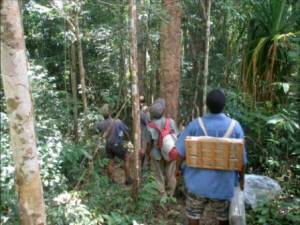
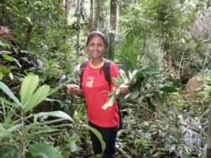
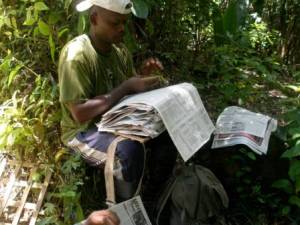
Abstract

The constantly developing uses of herbarium resources and advances in technology necessitate an update and partial revision of Chapter 27: Collecting Herbarium Vouchers of the Technical Guidelines. Examples of modern uses of herbarium specimens and associated data, and the application and methodology of new technologies are detailed and discussed. Several updates of the 1995 version of chapter 27 are provided, including some basic health and safety information. Anticipated future requirements and prospects for collectors of herbarium vouchers are briefly discussed. The gathering of high-quality herbarium-voucher specimens (particularly when they are accompanied with DNA samples and accurate georeference data) and related data are regarded as a critical and integral part of germplasm collection.

 

Introduction

The role of herbarium-voucher collectors has expanded considerably since 1995, due to improvements in technology, the emergence of new scientific methodologies and the extension of scientific and practical uses for herbarium vouchers and related data. Electronic equipment, such as global positioning systems (GPS), digital cameras and computers, have all become smaller and lighter, and battery life has improved. This has enabled herbarium collectors to take many new devices into the field as part of their everyday equipment, extending the amount and quality of the data that can be gathered. The use of DNA sequencing, and other molecular methods, utilized for a wide spectrum of scientific enquiries (population genetics, systematics, biogeography, rapid diversity assessments), has developed immensely since 1995, so that for many collectors, DNA sampling is now considered part of their regular protocol. The very nature of herbarium specimens, as permanent and verifiable records of organisms in space and time, makes them a fundamentally useful resource for several fields of enquiry, extending their use and value very much beyond their original and primary remit of taxonomy and systematics. Voucher specimens, in conjunction with accurate locality (georeference) data, are now also being used as the primary resources for conservation and diversity assessment (e.g., Golding 2004; Lister et al. 2010; Rivers et al. 2010; Roberts et al. 2005; Rondinini et al. 2006; Willis et al. 2003;), niche modelling, predictive mapping (e.g., Graham and Hijmans 2006; Phillips et al. 2006) and climate change (e.g., Pearson and Dawson 2003; Primack et al. 2004; Raxworthy et al. 2008). In order to maximize the potential of new technologies and novel scientific methodologies, for genebanking and germplasm science and the development of crop genebank management, it has been necessary to update and extend conventional protocols for voucher collecting. This information is outlined below.

 

Current status

New technology and equipment

Global positioning systems (GPS)

The latest generation of GPS units is lightweight, extremely accurate, has a long battery life and is capable of storing and downloading large amounts of georeference data. Earlier systems (mainly pre-2006) did not work well under the tree canopy, requiring the user to place the unit above or close to the canopy or to seek higher ground. In many cases, this considerably reduced the accuracy of readings, and users were often likely to take fewer georeferences. In May 2000, the degraded accuracy (about 100m) of civilian GPS was removed, increasing accuracy to about 15m. By 2006/7 most GPS units were fitted with highly sensitive receivers, more advanced microchips, and ground and space augmentation systems (“EGNOS” in Europe, “WAAS” in North America and “MSAS” in Japan). These changes have increased the accuracy to around 3m or better, with 95% confidence, given good satellite coverage. A good-quality modern GPS unit will now take an accurate reading under the tree canopy and in other previously problematic locations, such as in ravines and valleys. The long battery life means that multiple (e.g., 100s) of data points can made on a daily basis, and the unit can be left switched on for hours instead of minutes. Many collectors will now make an extended series of data points, capturing not only the exact position at which their herbarium vouchers were collected but also many other features, including records of absence, roads and paths, limits of primary vegetation (forest, native grassland), new villages and other settlements, and changes in land use. Most GPS units feature a track-log function, which will record the whole collecting journey in space (location) and time, which is an excellent means of geo-tagging specimens and photographs. These data are easily downloaded and stored electronically for later use in conjunction with global information system (GIS) software.

The most readily accessible and easiest tool for mapping your data is GoogleEarth™, which enables free and easy access to recent high-resolution satellite imagery, in conjunction with numerous tools and applications. The georeference data, or data points (also known as “waypoints”), are easily plotted manually, one by one or in large numbers, showing, for example, the route and extent of a collecting mission. In the first instance, this tool enables collectors to visualize their data points, check for accuracy and see whether they have applied the correct methodology for collecting the required spatial data.

All GPS units come with detailed instructions; the user needs to be familiar with the unit before collecting. Most important, the unit should be set up/configured for use in the correct manner. In most cases, the units should be set to metric, so that the data produced is given in metres (altitude) and kilometres (distance) and the time is set to local, although the latter is often set automatically. For the georeferences, the most common format is to set the GPS unit at degrees, minutes and seconds (e.g., N 49˚ 21ʹ 41.4ʺ E 30˚ 6ʹ 22.0ʺ) or degrees and decimal minutes (e.g., N 49 21.690 E 30 06.367). The former is preferred for herbarium voucher labels and, as good practice, should be copied into the field collecting notebook at the point of voucher collection.

The GPS unit will usually store the data in various ways, but the most useful for the user will be digital latitude and longitude (e.g., 49.36151 and 30.10612), which is used by most GIS software. Setting the GPS unit to the correct datum is essential. The World Geodetic System 1984 (WGS 84) is probably the most common datum for GIS data sets and is the one used for visualization with GoogleEarth™. Because the Earth is misshapen, when creating a datum to suit a specific country or region, geodesists have a “local” or “regional” datum. For some mapping projects, the use of the correct regional datum is critical, so consultation with project partners or the project manager on this point is very important. It is essential to note the datum used, even if it is WGS 84. It should also be noted that even when using local datum, the GPS unit might also record and store data in WGS 84.

Any investigation involving spatial analysis of distribution data necessitates accurate georeferencing of specimens, which in turn means that the collector of voucher specimens should be adequately trained and provided with the right equipment.

Digital Cameras

The advent of reasonably priced and easy-to-use digital cameras has accelerated the amount of imagery now available for understanding and visualizing germplasm and its natural environment. In conjunction with the voucher specimen, images can improve the chances of accurate identification by providing details of shape, colour and form, which are mostly lost when herbarium specimens are made. Other images can also be captured, such as habitat, associated species and possible threats to the population or individuals. Both types of images provide useful resources for publicity and media use. As with all other voucher information, it is important for the images to be linked to the voucher specimen by a unique identifier (e.g., the collector’s name and number, or a barcode), which in turn will provide a link to associated data, the most important of which is the accurate locality reference. Some cameras have a GPS processor as part of the unit; some GPS units incorporate a camera. It is also possible to geo-tag images using the GPS track log facility, linked to a digital camera, and there are numerous packages and software programmes available to do this.

Computers

Reasonably priced laptops, electronic notebooks and tablet computers are now widely available, and some have the additional advantage of long battery life. They all provide a means of recording and storing data directly in the field, with the possibility of linking to various software packages and the internet. In particular, many collectors like to download their photographic images on a daily basis, to free up camera memory cards, provide a back-up system and as a means of editing images. Hand-held data recording devices have been available for several years, performing similar functions as traditional notebooks but with added electronic functionality. Such devices have not yet replaced the field notebook, however, and field-testing during extended field studies suggests that they are currently of rather limited application. The main problem, and one that is common to electronic devices, is battery life, and the need for constant recharging, which is a particular problem where there is limited access to a reliable power source. However, with the advent of smart phones and similar technology, these problems will no doubt soon be overcome.

Other

Water- and solution-tight resalable bags, such as Whirl-Pak®, are now widely used for collecting spirit material in the field. These bags have the advantage that numerous spirit collections can be carried in a much smaller space, compared to rigid plastic bottles. Moreover, the close contact of plastic with sample means that very little spirit has to be used. Once the plant tissues have totally absorbed the spirit, the samples can be maintained for a few weeks with very little liquid, which is particularly important for transportation by plane. The spirit should be drained from the bag and the bag resealed; then several samples can be placed in a larger bag, the latter being totally sealed with non alcohol-soluble tape. Once the samples arrive at the herbarium or place of permanent storage, they can be decanted into a suitable archival liquid (Copenhagen Mixture or Kew Mixture) in appropriate storage jars (see Foreman and Bridson 1992).

DNA sampling

Before 1995, DNA samples would usually only be collected as part of a specific request or for target groups. With the increased demand for DNA samples, many collectors are now routinely collecting high-quality DNA samples for each herbarium voucher. If not required for an ongoing study, the DNA samples are banked in long-term storage facilities, either as silica-dried leaf material or as purified extracted DNA, for later use. Some herbaria now list their DNA sample collections via the internet so that researchers can access material that would otherwise not be available to them. The methodology for DNA sampling has not changed essentially since the silica-dried methodology was formalized (Chase and Hills 1991), although there has been a shift from collecting relatively small (less than 1g of fresh leaf material) to larger amounts of plant material for DNA extraction. This is due to the realization that samples might have to be used for multiple analyses under different protocols, and the advent of next-generation sequencing, all of which require more DNA. For this reason, it is often advisable to collect at least 2g–6g of fresh leaf material, depending on the plant and the methods being employed. A simple method for the collection of leaf material (adapted from Chase and Hills 1991) is given below.

Fresh leaf material is torn into small pieces (not exceeding 2cm²), to a total 4g–10g, and placed in small (12cm x 8cm) sealable plastic bags containing 50g–100g of fine-particle silica gel, including some indicator silica gel (which will change colour when wet, indicating whether the samples are rehydrating by absorbing moisture from the atmosphere). The ratio of fresh leaf material to silica gel should be about 1:10. Shake the bags to distribute the silica gel between the layers of leaves. If leaves are not completely dry within 12 hours, remove the silica gel and add an appropriate amount of new silica gel. Good-quality silica gel can dry 6 to 8 samples before being saturated.

To assess whether a leaf sample is thoroughly dry, bend one of the leaf pieces: if it is dry, it should snap and break cleanly. The leaf material may now be removed from the silica and placed in a new sealable plastic bag, or similar holder, with a small amount of silica gel, including some indicator type. The remaining silica gel can now be reused but must be checked very carefully to make sure that all fragments from the previous sample are removed. As the capacity of the silica gel is used up (i.e., as it absorbs water), the pieces of indicating gel turn from a dark violet-blue to pale blue and finally to a pale pinkish purple, or from amber to pale yellow, depending on the type of indicator gel used. At this point, the silica gel can be regenerated in an oven at 175˚C for one hour. It may also be dried using other heat sources, although longer periods of heat exposure are required (4 to 5 hours, overnight, or 1 to 2 days, depending on the heat source). The indicator silica gel should return to its original colour when regenerated.
Silica gel is an irritant, especially to the respiratory tract, and can cause irritation of the digestive tract. Fine-particle silica gel causes irritation to the skin and eyes. There are also long-term health issues associated with its use. For this reason, avoid contact with the skin, and only use it in a very well-ventilated environment. In addition, the blue indicator gel contains cobalt, which has also been associated with long-term health issues.

Other updates and comments on the previous (1995) version

Basic equipment for herbarium collecting

In addition to the basic equipment for herbarium collecting given in box 27.1 of the 1995 version of this chapter, it is good practice to include the items of equipment shown in the box below, which are divided into two categories: consumables and non-consumables. This does not include camping equipment, other field apparatus and safety equipment.

Preparing material in the field

In addition to the notes on preparing material in the field in the 1995 version of this chapter, it is strongly recommended that for larger samples, such as trees and shrubs, where a shoot or branch is selected as the specimen, at least one leaf be turned over so that the under-surface of the leaf is exposed. This is done by twisting the leaf at the petiole and then applying pressure after the pressing paper (e.g., newspaper) has been folded over the plant. Done in this way, the specimen will not have to be harshly manipulated prior to herbarium mounting. The under-surface of the leaf is often critical for correct species identification. For smaller plants, where more than one individual is collected per specimen, a whole plant can be turned over at the time of mounting.

Generally, any material over 3cm thick, such as wood and large fruits, should not be placed in the press, as it will cause the other specimens to become misshapen upon drying. Instead, such material should be wrapped in newspaper, or similar material, and placed separately on the plant drier. As with all voucher parts, this material should be numbered with a unique identifier (e.g., collector’s name and number), using a jeweller’s tag and/or written on with a pencil or permanent non-alcohol-soluble marker.

 

Basic Equipment for Herbarium Collecting Consumables Large (90cm x 60cm) heavy-gauge (500+) clear plastic bags (used to temporarily hold the plants until they are ready to prepare and press) New, large (90cm x 60cm) heavy-gauge (500+) clear plastic bags* Durable (waterproof) pocket-sized field notebook(s) for use with a pencil Several pencils (HB to 2B) and a sharpener Large and small, waterproof and non-alcohol-soluble marker pens (e.g., Sharpie® brand) Newspapers and corrugated cardboard sheets (43cm x 28cm) (required for preparing specimens for the Schweinfurth method and conventional air drying) Alcohol (preferably ethanol), 60%–70% (or higher that can be diluted to 70% in the field)* Good-quality plastic parcel tape or other non-alcohol-soluble tape* Parcel string Recommended or essential, depending on the project Whirl-Pak® plastic bags or similar for collecting spirit material Wide-mouthed plastic bottles (assorted sizes), such as Nalgene®, for collecting spirit material 70% ethanol or other temporary preserving fluid, for collecting spirit material Small bags (Ziploc® type) for silica gel DNA samples Silica gel Small (10cm x 7.5cm), medium (20cm x 19cm) to large (35cm x 20cm) bags (Ziploc® type), for various applications Rice sacks and rice sack needle (useful if bundling lots of alcohol-processed specimens, see below) Note: A good supply of all of the above items is required, the amounts of which should be carefully calculated according to the number of specimens anticipated. * Only required if Schweinfurth (alcohol) method is being used.

Non-Consumables Professional plant press(es) with heavy-duty straps A sharp pocket knife Scissors Hand lens (magnification x10) Tape measure or ruler Global positioning system (GPS), preferably including a barometric altimeter Mechanical altimeter Recommended or essential, depending on the project Digital Camera for recording appearance of the live plant, habit and habitat Batteries (for digital camera) or alternative power source(s), such as solar charger Small field binoculars (for looking into the tree canopy, etc.) Pole clippers/pruners (essential if collecting trees or where tree climbers are unavailable) Machete/parang (required if bark and “slash” information is needed) Heavy-duty thorn-proof gloves (if dealing with spiny plants such as rattans) Sturdy boxes for specimen transportation (required if plants are dried in the field)

 

Drying specimens

In addition to the notes on drying plant specimens in the 1995 edition of this chapter, the following information is given for completeness. Many collectors now use naked flames (including gas, charcoal and spirit burners) to dry plant specimens, particularly in remote areas. These methods come with inherent risks, as drying papers and plant material are readily combustible, particularly when previously treated with alcohol. Thus, the following information also includes notes on safety. A useful guide on collecting herbarium specimens is provided by Carter et al. (2007), with illustrations that demonstrate many of the main points given below.

1. Plant presses should be made up in the following sequence: corrugate – blotter (drying sheet) – specimen (between a sheet of folded newspaper) – blotter – corrugate – blotter – specimen – blotter – corrugate,…etc. Always end with a corrugate, which goes directly against one side of the press. The folded side of the newspaper should be lower-most in each press, so that no plant material can fall out of the press (and onto the heat source). Each press may be made quite large, but it should not be unstable or overly bulky; there should be nothing (such as specimen parts) sticking out of the press. When metal corrugates are used, the press size can be extended to the limits of the straps. If metal corrugates are not available, corrugated cardboard can be used, although then the press size will have to be much smaller, because the airflow with cardboard is considerably less and the plants will not dry properly.

2. The straps should be fastened as tightly as possible: tighten the first strap moderately firmly, fully tighten the second strap, then return to the first strap and fully tighten. If the straps are fastened in opposite directions, the pressure will be more even, although this not always the case. The long slats of the plant press should be outermost when the press is assembled and tightened, so that even pressure is applied to the specimens. (In most cases this will also avoid damage to the press.)

3. Expose the presses to a gentle (35°C to 45°C) heat source for as long as is necessary to dry the specimens properly, but they should not be over-dried or brittle. A variety of heat sources can be used in the field (e.g., gas, oil and charcoal heaters). Where there is a permanent facility, purpose-built and thermostatically controlled, fan-assisted drying ovens are the best, although alternative set-ups using electric fan heaters, electric elements and gas stoves can be adapted. A steady flow of warm air around and through the presses (via the corrugates) is just as important as temperature. Excessive initial heat can cause specimens to become “stewed” (recognized by discoloration and a “cooked cabbage” smell), especially if the drying papers are not frequently changed or if the plant is succulent. Some collectors warn against rapid drying, but generally it is considered desirable. The presses (and any loose material) must be well supported so that they cannot fall onto the heat source and start a fire. Make sure that the straps are securely tucked away so that they do not hang down and catch fire.

4. Each press should be examined regularly for tightness and turned so that the heating is even, although the edges of the newspaper should still remain lowermost. If allowed to become loose, undue distortion or shrivelling will occur, which might result in items being lost or falling onto the heat source. If necessary, a second folder of newspaper may be added to each specimen (the opposite way around) at the time of pressing. Examine the press at least twice a day and change the blotters (drying papers) as necessary, but not the flimsies. The dry specimens should be removed as soon as possible and the blotters (drying papers) made ready for re-use. Allow 18 hours to four days (or more) for complete drying. The specimens should be rigid when dry, unless very delicate. If possible, allow about 12 hours before handling the specimens after drying, especially for specimens prepared using the Schweinfurth (alcohol)

Equipment for drying specimens in the field

Two comments on box 27.2 in the 1995 version of this chapter are required:

• Newspaper is not the best type of drying paper (blotter). Thick blotting paper, or similar paper, 1mm–3mm thick, is preferable.

• If plants are dried in the field, as opposed to the Schweinfurth (alcohol) method, they will be brittle and very fragile after drying. In this case, sturdy boxes are required for carrying the dried plant specimens out of the field and for later transportation.

Chemical treatment: the Schweinfurth (alcohol) method

Additional comments for this section are also necessary. It should be pointed out that once the collector has access to plant-drying equipment, the alcohol-treated specimens can be carefully removed from the plastic bags and then dried in the conventional manner (see the 1995 version of this chapter 27 and the text above on drying specimens). Polythene tubes, as recommended in 1995, are generally not easy to obtain and, therefore, large (90cm x 60cm) heavy-duty (500+) clear plastic bags can be used – and in many cases are preferable. Inferior quality plastic bags can come apart at the seams if they are exposed to alcohol, so it is always a good idea to seal the seams with strong, non-alcohol-soluble parcel tape.

The most convenient way to tie up the bundles of plants, prior to placement in a plastic bag and wetting with alcohol, is to tie them with parcel string, using the “herbarium knot” (Forman and Bridson 1992). Roughly pillow-sized bundles are about right. It is important to wet all the specimens with alcohol, but the bundles should not be heavily saturated: any alcohol not absorbed within 10 to 20 minutes should be poured off. Likewise, always check the inside of the bundle to make sure that the flimsies (e.g., newspaper folders) are not dry. If they are, add more alcohol. It is good practice to add alcohol to the centre of the bundles first and let it absorb outwards through the bundle. Three or four bundles can be placed in a 90cm x 60cm plastic bag, which should be securely sealed with tape after removing as much air as possible. In difficult terrain or on long journeys, it always a good idea to double-bag the main plastic bag. Two or more completed packages can then be placed in a rice sack for extra durability and ease of transport. It is also advisable to keep the packages out of direct sunlight. Properly prepared and carefully stored Schweinfurth-prepared specimens will last for many months prior to drying.

Recording data

In addition to recording the features of the plant (see 1995 chapter), it is essential (for the production of herbarium labels and for subsequent scientific analysis) for all the basic information to be recorded at the time of collection. The following guidelines are provided:

Information Required for Each Specimen Entry, Where Applicable A specimen is only useful if it is accompanied by adequate field notes and has a unique identifying number to accompany it. The best system of unique identification is a consecutive number series for each collector. This should start at 1, and each number should refer to only one collection, and never be repeated. Therefore, the collector’s name(s) + their collection number comprise the unique identifier. For common surnames, or where joint collectors have the same surname, initials are used to provide the specimen with a unique identifier (e.g., Jones [W.P.] 14962; Dransfield [J.] & Dransfield [S.] 17346). All duplicates (parts of the same plant) should bear the same unique identifier. Collectors name(s) and number (see above) Precise location: country, state/province/division (or any meaningful/useful division or divisions within the country); kilometres and direction from an obvious landmark (e.g., town, large village, mountain summit, river mouth); georeference (latitude and longitude) recorded with a GPS (set GPS to degrees, minutes, seconds; and metric units) Altitude: record with mechanical altimeter, equilibrated against a known altitude (i.e., sea level) (Some modern GPS units have accurate barometric altimeters.) Habitat: Vegetation type (humid, evergreen forest, mangrove, savannah) (If possible add dominant species to more precisely indicate vegetation type/association.) Geology: rock or substrate type (This is not always possible if the soil is thick or if geology is complex.) Soil type (iron-rich, silty, sandy) Other: topography, slope, exposure Plant description: record features that will not be present or evident from the dried pressed specimen (tree, shrub, or herb; height; shape, structure, architecture); notes on root system; features that may be lost on drying (e.g., colour of flower parts and other parts that are coloured); odour (flowers, leaves, wood and bark); exudates, oils and waxes; if it is a tree or large shrub, record the bark characteristics (texture, slash, exudates) and diameter at breast height (dbh) Date of collection: use a system that is unambiguous (e.g., 21 Aug. 2008) Associated material: if the main specimen is accompanied by additional items that will be linked together at a later date, record these in the notebook; e.g., photographs (image number can be recorded in notebook), fruit (carpological specimen), DNA samples, spirit material, wood sample, ethnobotanical artefact, medicinal product Number of duplicates: record the number of duplicates that have been collected for each accession number Additional collectors: note the full names or surname plus initials of the collecting team; for ethnobotanical collections or when vernacular names are being collected, be sure to record the language used, village/tribal affinities (if relevant) and the name of the informant

Storing and dispatching vouchers

In the 1995 version of this chapter, the use of para-dichlorobenzene (i.e., moth balls) prior to storage and dispatch is recommended as an effective deterrent against pests. Although there is no direct evidence, para-dichlorobenzene may be reasonably anticipated to be a carcinogen, and it is banned by some institutes. Likewise, naphthalene is classified as possibly carcinogenic to humans and animals, and exposure to large amounts may damage or destroy red blood cells.

 

Future challenges/needs/gaps

Developments in the use and application of herbarium data have extended the role and value of this recourse for germplasm science and genebanking. Today’s collectors need to be aware of these changes so that they can develop their equipment and protocols accordingly. This is particularly true for the collection of DNA samples and the use of new electronic equipment, especially geo-location hardware (GPS) and GIS software. At present, the use of some electronic equipment, such as portable computers, is limited by battery life and problems with recharging in the field, although these issues will no doubt be overcome. GPS devices will become more accurate and increasingly sophisticated. Hand-held electronic notebooks and other data-recording devices have improved and may become mainstream in the future. Protocols for long-term storage of silica-dried and extracted DNA material requires further investigation and investment, including looking into aspects related to data-basing and future access. As with all extra-locally gathered resources, further work on prior informed consent, access and benefit-sharing agreements is also required. One of the biggest challenges for the future, however, is the maintenance and development of herbaria and other voucher storage facilities, which include the training and retention of skilled curators and specimen-based scientists.

 

Conclusions

The collection of herbarium-voucher specimens and associated data is an integral component of germplasm collection and genebanking, and where possible, best-practice procedures should be followed and maintained. Developments in the use and application of herbarium data have extended the role of these resources, and the modern herbarium-voucher collectors will need to be aware of these changes so that they can develop their equipment, skills and protocols accordingly. The value of high-quality, accurately georeferenced herbarium specimens and associated material, particularly DNA, should not be underestimated.

Back to list of chapters on collecting

 

References and further reading

Carter R, Bryson CT, Darbyshire SJ. 2007. Preparation and use of voucher specimens for documenting research in weed science. Weed Technology 21:1101–1108.

Chase MW, Hills HH. 1991. Silica gel: an ideal material for field preservation of leaf samples for DNA studies. Taxon 40:215–220.

Foreman L, Bridson DM, editors. 1992. The Herbarium Handbook. Revised edition. Royal Botanic Garden, Kew, UK.

Golding JS. 2004. The use of specimen information influences the outcomes of Red List assessments: the case of southern African plant specimens. Biodiversity and Conservation 13(4):773–780.

Graham CH, Hijmans RJ. 2006. A comparison of methods for mapping species ranges and species richness. Global Ecology and Biogeography 15:578–587.

Lister DL, Bower MA, Jones MK. 2010. Herbarium specimens expand the geographical and temporal range of germplasm data in phylogeographic studies. Taxon 59:1321–1323.

Pearson RG, Dawson TP. 2003. Predicting the impacts of climate change on the distribution of species: are bioclimate envelope models useful? Global Ecology and Biogeography 12:361–371.

Phillips SJ, Anderson RP, Schapire RE. 2006. Maximum entropy modeling of species geographic distributions. Ecological Modelling 190:231–259. Available online (accessed 6 October 2011): www.cs.princeton.edu/~schapire/papers/ecolmod.pdf.

Primack D, Imbres C, Primack RB, Miller-Rushing AJ, Del Tredici P. 2004. Herbarium specimens demonstrate earlier flowering times in response to warming in Boston. American Journal of Botany 91:1260–1264.

Raxworthy CJ, Pearson RG, Rabibisoa N, Rakotondrazafy AM, Ramanamanjato J-B, Raselimanana AP, Wu S, Nussbaum RA, Stone DA. 2008 Extinction vulnerability of tropical montane endemism from warming and upslope displacement: a preliminary appraisal for the highest massif in Madagascar. Global Change Biology 14:1–18.

Rivers MC, Bachman SP, Meagher TR, Lughadha EN, Brummitt NA. 2010. Subpopulations, locations and fragmentation: applying IUCN Red List criteria to herbarium specimen data. Biodiversity and Conservation 19:2071–2085.

Roberts DL, Moat J, McInerny GJ. 2005. What have herbaria ever done for us? The role of herbaria in conservation assessments. Selbyana 26:299–303.

Rondinini C, Wilson KA, Boitani L, Grantham H, Possingham HP. 2006. Tradeoffs of different types of species occurrence data for use in systematic conservation planning. Ecology Letters 9:1136–1145.

Willis F, Moat J, Paton A. 2003. Defining a role for herbarium data in Red List assessments: a case study of Plectranthus from eastern and southern tropical Africa. Biodiversity and Conservation 12:1537–1552.

 

Back to top

Chapter 26: Collecting symbiotic bacteria and fungi

L. Herrmann
TSBF-CIAT, World Agroforestry Centre, Nairobi, Kenya
E-mail: l.hermann(at)cgiar.org
D. Lesueur
TSBF-CIAT, World Agroforestry Centre, Nairobi, Kenya, and
CIRAD, UMR Eco&Sols (CIRAD-IRD-INRA-SupAgro) Land Development Department, Bangkok, Thailand
E-mail: didier.lesueur(at)cirad.fr

Online resources (annex 1) compiled by:
F. Giampieri
Bioversity International via dei Tre Denari 472/A 00057 Maccarese, Rome, Italy
E-mail: f.giampieri(at)cgiar.org

	2011 version (0.7 MB)	1995 version (0.3 MB)
	Open the full chapter in PDF format by clicking on the icon above.

This chapter is a synthesis of new knowledge, procedures, best practices and references for collecting plant diversity since the publication of the 1995 volume Collecting Plant Diversity; Technical Guidelines, edited by Luigi Guarino, V. Ramanatha Rao and Robert Reid, and published by CAB International on behalf of the International Plant Genetic Resources Institute (IPGRI) (now Bioversity International), the Food and Agriculture Organization of the United Nations (FAO), the World Conservation Union (IUCN) and the United Nations Environment Programme (UNEP). The original text for Chapter 26: Collecting Rhizobium, Frankia and Mycorrhizal Fungi, authored by R. A. Date, has been made available online courtesy of CABI. The 2011 update of the Technical Guidelines, edited by L. Guarino, V. Ramanatha Rao and E. Goldberg, has been made available courtesy of Bioversity International.

Please send any comments on this chapter using the Comments feature at the bottom of this page. If you wish to contribute new content or references on the subject please do so here.

Back to list of chapters on collecting

References for this chapter

Annex 1: Internet resources on collections of microbial cultures

 

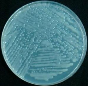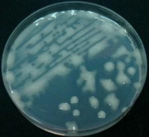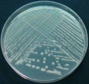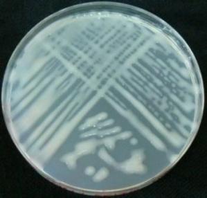	Microorganisms (Photos: L. Hermann/CIAT-TSBF)

Abstract

Soil is the habitat of an array of microorganisms in all three taxonomic domains. Because many species of soil microorganisms are still unknown or non-described, the assessment of microbial diversity, especially the symbiotic bacteria and fungi is not feasible undertaking. In designing field sampling to collect symbiotic microorganisms, the challenge is to select a subset of the soil biota that adequately reflects the anticipated taxonomic spectrum, and which at the same time includes all the symbiotic microorganisms considered important. Designing a successful, practical sampling scheme is an art. In this chapter, we tried to provide a guideline to make it correctly ensuring the representative of all the indigenous symbiotic bacteria and fungi naturally present in the soils of sampled sites. As the majority of the microorganisms, including the symbiotic ones, are found in the upper 20cm of the soil profile, the main investigations have to be done on topsoil even if it doesn’t mean that microorganisms are not naturally present in deeper layers. Once the samples have been harvested, it is important to be cautious and store them nicely for further microbial analysis. Otherwise the risk to lose them or to get only contaminants after streaking is pretty high. This chapter describes some protocols and methodologies with practical and simple recommendations easily repeatable by people who have interest to make such laboratory work. We tried to raise the main steps ensuring the success of the establishment of the collection of symbiotic bacteria and fungi coming from all around the world.

 

Introduction

Symbioses between higher plants and bacteria or fungi are known to be important, and perhaps essential in some cases, for good plant growth. This is generally recognized to be due to improved nutrition of the host plant. In the case of the legumes for instance, the nitrogen nutrition of the plant relies on the symbiotic rhizobia that are able to fix nitrogen from the atmosphere through biological nitrogen fixation (BNF). BNF is one of the most important processes for the maintenance of life on earth, as it contributes about 70% of all nitrogen required by natural and agricultural ecosystems and is environmentally friendly. In Brazil, for example, inoculation with Bradyrhizobium strains has completely replaced the application of chemical fertilizers for soybean. In 2006, with a soybean yield of 57 million tuns, about US$ 3.3 billion in fertilizer expenses were saved because of this biotechnology (Moreira 2008).

Satisfactory exploitation of new plant germplasm in new environments may depend on the natural presence of a suitable microsymbiont or its simultaneous introduction. Microsymbionts are widely distributed around the world, but that does not mean that all of them are compatible with different legumes and crops. Experience suggests that there is a close genetic association between host plant and microsymbiont (Sprent 2009). Thus, when plant germplasm is being collected for use in new environments, it is recommended that symbiotic microorganisms also be collected. It is very important to collect and identify microsymbionts coming from several agroecological zones (AEZ) in order to get those capable of forming an effective symbiosis with the targeted host plants.

The most important microsymbionts include the following:

• the root-nodule bacteria or rhizobia that form nitrogen-fixing symbioses with legumes, currently including 50 species distributed among the genera Rhizobium, Ensifer, Mesorhizobium, Azorhizobium and Bradyrhizobium (Velasquez et al. 2010)

• Burkholderia, which has only recently been recognized as a potential nitrogen-fixing symbiont of legumes, especially Mimosa (Bontemps et al. 2010)

• the vesicular arbuscular mycorrhiza (VAM) for phosphorus supply in many plants (Habte 2006; Varma 2008)

• the actinorhizal associations (Frankia) for nitrogen supply in about 200 species, including forages and forestry species such as Alnus, Allocasuarina, Elaeagnus, Hippophae, Purshia and Shepherdia (Dommergues et al. 1998)

• the ectomycorrhiza (over 1000 species of Basidiomycetes and Ascomycetes, mainly the former) for water and nutrient uptake in many forest species in the families Pinaceae, Betulaceae, Salicaceae, Myrtaceae, Casuarinaceae and some Caesalpiniaceae and Dipterocarpaceae (Girlanda et al. 2007; Varma 2008)

Many of the early studies of inoculation with a microsymbiont involved the transfer of soil from established crops, plantations and forests. Today, most microsymbionts can either be cultivated on artificial media or maintained as “enriched” cultures in association with an appropriate host nurse-plant in controlled conditions. Molecular tools can be used to confirm that they are still genetically correct and correspond to the initial microsymbionts. These cultures provide a good source of inoculum that can be introduced into the soil with the seeds at sowing, applied either separately or directly to the seed or seedlings.

Some of the practical problems of collecting symbiotic microorganisms are outlined in this chapter as a guide to the collector of plant germplasm undertaking this work for the first time. The approach and methodologies described define principles and can be altered to suit individual requirements and facilities.

 

Current status

Pre-sampling considerations

Suitable isolates of the target microsymbiont may already be available. If potentially useful strains are not available, one must decide where to collect them. Prospecting for microsymbionts should concentrate on the same geographic and ecological areas from which the plant germplasm to be inoculated was collected.

Edaphic factors are particularly important in identifying areas where suitable strains would most likely be found (Date et al. 1979; Molina and Trappe 1982).

A perhaps more common situation, however, is for plant germplasm and microsymbiont collecting to occur in tandem. For example, a plant germplasm collector may also gather nodule samples and return them to a colleague in a microbiology department or institute for isolation of the microorganism. Joint collecting trips might be required when it is necessary to isolate organisms from fresh nodule or root material.

Ideally, the microsymbiont and seeds should be collected from the same plant. However, this is often difficult, since seed collecting is often best done at times when the host plant has a reduced complement of active nodules or mycorrhiza. For example, nodules from annual legumes are best obtained from seedlings, although the nodule population in young plants may be composed of a suite of strains different from that of older (seed-producing) plants, as seasonal and soil conditions change (Caldwell and Weber 1970; Weber and Miller 1972; R.A. Date, unpublished data for strains of Bradyrhizobium forming nodules on Stylosanthes). Another example is Leucaena growing as a closed-canopy stand. It has been observed to have nodules at 98 days but not at 205 or 274 days; nodules reappear on the root system at 423 days (Wong et al. 1989).

The presence of nodules on the root system in nitrogenfixing symbioses is often seasonally dependent, especially if soil nitrogen is at levels adequate for good plant growth. In long-lived perennial plants, for example, maximum seed set is often in the dry season, when nodules and fungi are not easily found. Sampling of soil and roots for ectomycorrhizal organisms is best done in the spring, when plants are actively growing. Young sporocarps are preferred for isolation but it is important to collect fully mature material for reliable identification of the species. Ectomycorrhizal numbers and sporocarp production also vary seasonally (Grand and Harvey 1982).

Arrangements for the isolation and storage of the microsymbiont material should be made before setting out. When collecting abroad, it is essential to clear and coordinate microsymbiont collecting activities with the relevant local authorities, in the same way as it is done for plant germplasm. Microsymbionts are just as much a part of biodiversity as the plants on which they live. Material collected by a national programme in its own country may need to be isolated or stored abroad, if adequate facilities are not available locally, and the isolates re-imported as and when necessary. Quarantine clearance for the import and export of microsymbiont material may be necessary; this question should be investigated before setting out to collect.

Sampling strategy

The sampling strategy is key to successful collecting. There is a long tradition of sampling in field ecology, and hence much experience has been accumulated. In addition, there is a well-established theory of sampling that applies anywhere it is attempted (Cochran 1977). There are numerous texts describing both theory and application (Gregoire and Valentine 2007). Huising et al. (2008) described some of the options for sampling for below-ground biodiversity, including microsymbionts, and they listed the advantages and disadvantages of different approaches. These authors suggested the use of sampling windows: a rectangular parcel of land that includes the range of locally significant land uses for study considered “representative” of the site. A regular grid (with variable spacing) is used to identify a set of possible sampling points within each window; the points correspond to the intersections of grid lines. The total number of sampling points per site is between 100 and 120 points.

The distribution of microsymbionts may reflect landscape gradients (for example, those of soil organic carbon) and cultivation practices, or it might correlate with topography or vegetation patchiness or with soil resource gradients, or even with the location of the legumes. Spacing 200m between sampling points seems acceptable because it allows a relatively larger area to be covered by the grid and is more likely to reflect the most dominant land uses in the sample, while in most cases it is still possible to traverse from one point to the other.

Soil microorganisms such as microsymbionts respond to seasonal changes, and their diversity (richness and abundance) will show marked differences between the seasons. With respect to arbuscular mycorrhizal fungi, for example, the dry season is more favourable for the production of spores than the rainy season, and those spores are also the best preserved. For ectomycorrhizal fungi, the structures and reproductive cycles (e.g., formation of sporocarps) have evolved to be in synchrony with seasonal changes, and the best time to collect them is towards the end of the rainy season.

Collection of samples from the field

For rhizobia, legume species typical of the area should be selected for nodule sampling. Ideally, each sample of microsymbiont should be unique and originate from a single plant. It should also be associated with a single-plant seed sample, as symbiotic microorganism and host are often closely affiliated genetically. Experience has shown that 10 to 20 legume nodules per plant should be collected to adequately sample the variation in strain types in the nodule population. It is a good idea to collect two to five samples to represent a single site, as not all nodules will yield a viable culture and only a small proportion (as low as 5%) of the nodules may contain an effective nitrogen-fixing strain.

Similar guidelines apply to collecting Frankia, VAM and ectomycorrhizal fungi. Usually, it is only necessary to process about half the sample, keeping the other half as a reserve against accidental loss during surface sterilization and isolation.

It is important in collecting microsymbionts to know where to look on or about the root system for nodules, rhizomorphs and sporocarps. The location of nodules on the root system is very species-specific and is further influenced by local conditions. In small, strongly tap-rooted species like Trifolium semipilosum, nodules can be found within 4cm to 5cm of the root crown. In Stylosanthes, nodules are more or less equally distributed along the length of the root system to a depth of 15cm, but may be deeper in species like S. capitata growing in acid sandy soils (Venezuela) or oxisols (Brazil). Acacia and Casuarina species growing in free-draining deep sands have nodules at depths of 1m–2m, which is probably related to the level of the water table.

Small herbaceous legumes (e.g., Trifolium semipilosum, Lotus spp.) can be sampled by digging a small core (diameter 10cm–15cm, depth 10cm) around the top root. For shrubs and trees, it is rarely necessary to excavate the entire root system. Careful removal of soil from around the root crown with a knife or small trowel usually provides good results. Most nodules are located on adventitious roots in the top 5cm of soil. For seedlings, a small core (as for herbaceous legumes) of soil around the root is usually adequate, but on mature plants, nodules may be found further out and much deeper, depending on conditions. Usually, it is possible to collect nodules from the cores by sequentially fragmenting the soil by hand, but it might be necessary with dry or clay soils to soak the core of soil in water and allow the soil to fall away. Alternatively, and especially in species where nodules become detached readily from fine adventitious roots (e.g., Macroptilium, Leucaena), soil and roots with nodules can be washed over a sieve (1mm–2mm openings). In either case, nodules can be recovered with forceps.

Nodule size and shape are also very species-specific. Those of Arachis and Stylosanthes are 1mm–2mm in diameter and firmly attached, whereas those of Alnus, Casuarina, Macroptilium and Medicago are typically larger and become detached readily. The shape of legume nodules is governed by the extent and location of the meristem. Hemispherical peripheral meristems produce spherical nodules, as typified by Arachis, Glycine, Lotus, Macroptilium, Stylosanthes and Vigna.

Nodules on most non-leguminous plants are modified lateral roots with slow-growing meristems, usually branching dichotomously to give coralloid-type nodules up to 5cm–6 cm long, as typified by Alnus, Casuarina and Ceanothus (Becking 1977).

Endomycorrhizal plants have no obvious macroscopic structures, but with experience, hyphal growth on the roots may be recognized with a hand lens. There is wide variation in the morphology of ectomycorrhiza. They appear as a continuation of the root in Pinus taeda, but coralloid forms on P. strobus and P. resinosa are more like the root nodules of Lupinus (Grand and Harvey 1982). In other host species, the mycorrhiza varies from a thin mantle of fungal hyphae to thickened zones of terminal roots (Chilvers and Pryor 1965). In Acacia and Nothofagus species, gasterocarps up to 3cm in diameter may be found in the top 10cm of soil, usually on the side exposed to the prevailing winds, within 1.5m of the trunk. They are usually most plentiful in late autumn, winter and early spring (Beaton et al. 1985)

Box 26.1: Equipment required for collecting microsymbionts Digging implement (trowel, strong knife) Secateurs or strong scissors Forceps, scalpel or small sharp knife Hand lens Collecting vials with desiccant Waxed paper bags Paper towels 5-litre plastic container Permanent marker pen Adhesive tape Plastic bags Containers for storage of samples Cooler box (optional) Note: See Date and Halliday (1987) for details of portable kits if isolation of microsymbiont is to be attempted in the field.

 

How to isolate microsymbionts according to the nature of the samples

Microsymbionts can be isolated from nodules, roots or soils. For the rootnodule bacteria of legumes and for many actinorhizal organisms, the best source is obviously nodules obtained directly from the plant from which seeds are also being collected. When nodules are not available, collectors should sample a small piece of root and/or soil from near the root. For rhizobia, the conventional method is to use promiscuous trap species to isolate indigenous strains from soil samples collected in the field. These can be used to inoculate seedlings of the host plant growing aseptically in order to obtain fresh nodules, from which isolates can be made. However, this is a method of last resort, because it will not necessarily yield nodules of those strains that would have formed in the field. This could be significant, depending on the exact purpose for which nodules are being collected. If, for example, specific collecting is being carried out for a strain with the ability to nodulate a host at low soil pH or for a strain that is highly competitive for nodule formation in the presence of large populations of ineffective strains, then reproducing these conditions for aseptically growing seedlings might not be possible. However the use of multiple trap species is not usually feasible with a large number of sampling points because of the laborious nature of the procedure and the limits of time and laboratory facilities. Therefore, a single promiscuous trap species is employed. In these circumstances, Macroptilium atropurpureum is a good choice, as it has small seeds and is easy to manipulate under controlled conditions in plastic pouches and Leonard jars in a growth chamber or greenhouse. According to Moreira (2008), when multiple experiments are carried out, seeds from the same accession should be used because this will avoid any possible influence of plant accession on indigenous rhizobia trapped.

Collecting soil and/or root pieces is the only way of obtaining material of those microsymbionts that do not form nodules or that cannot be grown easily in axenic culture (e.g., Glomus, VAM and some ectomycorrhizal organisms). In these cases, pure or enriched cultures may be obtained by collecting spores by a wet sieving method (e.g., Beaton et al. 1985; Gerdemann and Nicholson 1963; Hayman 1982; Molina and Palmer 1982).

For arbuscular mycorrhizal fungi (AMF), the utilization of the most probable number method described by Bagyaraj and Stümer (2008) is relevant. It consists of estimating the number of infective propagules of AMF in several soils by making a series of tenfold soil dilutions where presence or absence of mycorrhizal colonization is recorded and results given as a probability of the number of infective propagules based on a statistical table. The advantage is that the analysis of trap host roots to check is fast and easy to carry out and can also provide AMF material for further isolation of spores. Spores are the only part of the fungal organism that can be used to start aseptic cultures (hair-root cultures infected with AMF can also be produced and disseminated as starter cultures for further larger inoculum production). Spores are extracted from the soil by wet sieving followed by sucrose gradient centrifugation (Bagyaraj and Stümer 2008).

Storage guidelines

The viability of symbiotic bacteria and Frankia in the nodule sample is variable, and it is best to isolate on the day of collecting or soon thereafter. When this is not possible, nodules must be properly stored to ensure the viability of the cells they contained. Nodules are generally dried or kept frozen.

The microsymbiont will usually remain viable in the dried state for several weeks, with 75% to 90% of the nodules yielding viable isolates after reimbibition and surface sterilization. Drying is best achieved by placing nodules in an airtight vial or screw-capped bottle with a desiccant such as anhydrous CaCl₂ or silica gel (Date and Halliday 1987). Washing samples should be avoided, but, if it is necessary, then nodules should be dried with absorbent paper before being placed in the vial with desiccant. The desiccant can be kept in place by a plug of cotton or absorbent paper. Its volume should exceed that of the sample. A vial with a capacity of 10ml to 20ml, filled to 25% of its volume with desiccant and 10% made up of cotton or paper plug, is a good container for preserving and transporting samples. Vials should be kept cool.

As an alternative, the nodules may be surface sterilized and stored in glycerol at -20°C or -80°C. The methodology to use is as follows:

• After the nodules are collected from the plant, thoroughly clean them through sieves and store them in a refrigerator at 4°C, awaiting sterilization for long-term storage.

• Fill McCartney bottles or any other autoclavable bottles with enough glycerol to submerge all the nodules. If McCartney bottles are used, pour in about 10ml of glycerol and autoclave for 20 minutes at 121°C.

• Autoclave for 20 minutes at 121°C: the sieves, at least five bowls and distilled water.

• Prepare calcium hypochlorite 3.3% solution (or use commercial bleach) and 70% ethanol.

• For sterilization, place the sieve into the bowl of sterile distilled water and pour the nodules onto the sieve to rinse off any dirt. Remove stones, leaves or any other waste.

• Place the sieve with the nodules onto the first bowl with calcium hypochlorite for one minute and transfer it to the next bowl for another minute.

• Finally, transfer the sieve to the last two bowls of sterile distilled water in order to rinse the nodules.

• Using sterilized forceps or spatula (sterilized with ethanol and fire), transfer the nodules to the storage bottles containing sterilized glycerol solution 20%.

• The nodules can then be stored at –20°C and below.

• It is important to remember that reagents have to be regularly changed after several washes.

There are some species where the proportion of recovery is less than 5% of nodules and it is therefore necessary to isolate them from fresh nodules. For example, no viable isolates of Bradyrhizobium were obtained from more than 150 dried nodule samples of Stylosanthes capitata collected in Brazil and processed in Australia six to 10 weeks later, but isolation was 65% to 80% successful for fresh nodules processed the day of collection (R.A. Date, unpublished data). When isolations are to be made on the day of collection, the simplest method is to gather all or part of the root system into sealable polythene bags. On return to a laboratory, roots and nodules must be washed free of soil and the nodules excised with a short piece of root attached. Portable isolating kits are available and have been described by Date and Halliday (1987).

Unlike nitrogen-fixing root nodules, sporocarps should be kept dry, but not airtight. Waxed paper containers are usually used (Molina and Palmer 1982).

Isolation of microsymbionts

Successful isolation of microsymbionts depends on the quality of the sample. Damaged symbiotic bacteria or Frankia nodules are not satisfactory and should be used only to inoculate aseptically growing seedlings of the host plant to obtain fresh nodules. Dried nodules need to be reimbibed for 30 to 60 minutes before surface sterilization. Methods of sterilization and isolation vary with individual requirements and with the microsymbiont. A number of laboratory procedures have been described for the following organisms:

• Rhizobium, Ensifer, Mesorhizobium, Azorhizobium and Bradyrhizobium (Brockwell 1980; Date and Halliday 1987; FAO 1983; Moreira 2008; Somasegaran and Hoben 1985)

• Burkholderia (Bontemps et al. 2010)

• VAM (Bagyaraj and Stümer 2008; Daniels and Skipper 1982; Hayman 1982)

• Frankia (Diem and Dommergues 1983; Stowers 1987)

• Ectomycorrhiza (Molina and Palmer 1982)

To cultivate rhizobia, start by crushing one nodule according to the following methodology:

• Put the nodules in a plate containing 70% ethanol for 30 seconds.

• Using sterilized forceps (sterilized with ethanol and a flame), transfer the nodules to a 3.3% Ca(OCl)₂ solution for two minutes. After this step, the nodules are handled aseptically.

• Transfer the nodules to the subsequent plates in order to rinse them three times. Sterilize the forceps before every transfer.

• Under aseptic conditions, insert a nodule into a 1.5ml eppendorf tube.

• Add 200μl of sterile distilled water and crush the nodule using a sterile plastic pestle.

• If needed for further analysis of the microsymbiont, aliquot 50μl of nodule suspension into another eppendorf tube and add 50μl of 40% glycerol. Cover the cap with parafilm to prevent the tube from opening during storage and then store it at -20°C. This 50μl suspension can be used to isolate strains of rhizobia contained in the nodule.

• The rest of the nodule suspension is used for short-term analysis. If the analysis is not run immediately after crushing, tubes can be stored for a few days at 4°C.

Microbiological culture is a method of multiplying microbial organisms by letting them reproduce in predetermined culture media under controlled laboratory conditions. In theory, from a single cell, a population composed of millions of identical cells (identical to the mother cell) can be obtained. In a liquid medium, bacteria diffuse throughout the liquid: the growth results in a turbulent appearance of the medium a few hours to a few days after incubation at optimized conditions. On a solid medium, bacteria are not able to diffuse. The mother cell divides and the cells formed stay close to each other, forming a mass called a colony.

The following procedure describes how to cultivate bacteria in aseptic conditions, in accordance with good laboratory practice (GLP), from different kinds of samples, on a solid and/or liquid medium.

Box 26.2: Definitions Aseptic conditions/Aseptically: An aseptic environment is one where no microorganism is present. This can be obtained using a Bunsen burner (the aseptic zone is the spheric area around the flame with a diameter of approximately 15cm) or a laminar flow hood (sterile air is continuously produced and present in the hood; the difference in pressure between the inside and outside of the hood prevents the air outside from coming inside and contaminating the environment under the hood). Contaminated by microorganisms: Every plate, tube, pipette or other instrument (glassware, pestles, eppendorf tube, etc.) that has been in contact with microorganisms and which cannot be sterilized by the flame of a Bunsen burner is considered to be contaminated. Contaminated by toxic chemicals: Every tube, flask, pipette or other instrument (weighing boats, glassware, etc.) that has been in contact with toxic chemicals is considered to be contaminated. Good laboratory practice (GLP): The principles of GLP have been developed to promote the quality and validity of results and of the analysis conducted in a laboratory. It is a managerial concept covering the organization and the conditions under which laboratory studies are planned, performed, monitored, recorded and reported. Its principles also include the protection of humans and the environment. Mother tube/plate/product: This is the tube/plate/product from which the bacteria are picked. The result of the growth of this inoculation is considered to be the “daughter”, which can become the mother for the next inoculation.

 

Box 26.3: Materials, furniture, reagents 1. Chemicals - Mother plate/tube/product - Liquid media (tubes, flasks…) - Physiological water in tubes (NaCl, 9g/litre) - Sodium hypochlorite solution (JIK®) - Solid media (in plates or tubes) 2. Material - Bunsen burner - Incubators and rotative incubator - Laminar hood - Vortex 3. Instruments - Forceps - Loop - Mother plates, tubes or products - Plastic box for incubation - Racks for test tubes - Sterile Pasteur pipettes

 

Description of analysis

Preparation of media

Plates or tubes of media have to be prepared a couple of days before analysis. The medium is composed of nutrients, agar (if solid) or water at a specific pH. The composition of the medium depends on the target bacteria to be cultivated – to either enhance or inhibit the growth of certain bacterial groups. Some specific additives (such as vitamins, antibiotics, etc.) might also be included to create a more specific medium.

A solid medium is a gel matrix supporting the growth of many microorganisms, such as bacteria, fungi or yeasts. Liquid media are sometimes referred to as “broth” (e.g., nutrient broth). These are available for use in test tubes, bottles or flasks. In a liquid medium, bacteria grow uniformly, producing general turbidity. The composition is usually the same as for solid media in regard to the nutrients, but it does not contain any agar. The pH is also adjusted to provide good growth conditions.

Rhizobia are generally grown on a medium containing mannitol as the main carbohydrate source. Few groups of bacteria are able to use this sugar as their principal source of energy; their growth will be slowed while the growth of the rhizobia will be enhanced. The composition of this medium (yeast extract mannitol agar, YEMA) is as follows:

YEMA:
K2HPO4	(0.5g/litre)
MgSO4, 7H2O	(0.2g/litre)
NaCl	(0.1g/litre)
Yeast extract	(1g/litre)
Mannitol	(10g/litre)
Agar pH : 6.8	(15g/litre) (only if solid medium)

The medium is autoclaved for 20 minutes at 121^oC. Solid media have to be poured (in aseptic conditions) into Petri plates while still hot and liquid. The agar will become solid as it cools. Plates are left to set at room temperature and then turned upside down until use in order to avoid condensation at the surface of the gel. Liquid media (in tubes, flasks, etc.) can be kept at room temperature.

Bench organisation

The rack with the tubes or the plates from which the bacteria will be picked is placed on the side near the burner, with the pipettes or the loop on the opposite side. The rest of the bench has to be clear. Other plates and tubes, which are not being used, can be placed on the side of the bench (or on a trolley next to the bench) as far as possible from the place where you are working. Again, plates should be placed upside down. Anything not useful has to be off of the bench.

Usually, one plate is inoculated with one crushed nodule but several nodules from the same plant (or plants collected together) are analyzed and considered as replicates.

Preparation of “receptor” tubes or plates

All the plates and tubes have to be labelled before starting any manipulation. Note the date of the manipulation, the kind of sample you are using (name of the strain, origin, number of the sample, etc.) and any other information that might be useful. If many samples will not be incubated at the same temperature, also write the incubating temperature on the label. On the plates, write on the reverse side so that what is written can be read once the plate is incubated.

Sterilization techniques

The bacteria have to be picked up using a sterilized loop or pipette. To sterilize the loop, pass it horizontally through the blue flame (all of the metallic part), from the handle to the end (all the parts that might come in contact with the tube). Then put it vertically on the flame. The platinum loop has to become red hot. Let it cool down for a while before using it. If cottoned Pasteur pipettes are being used, break the end of the pipette (red mark) if needed and then sterilize the outside by passing it through the flame. Pass the pipette through the fire but not long enough for the glass to melt. Be careful not to contaminate the part that will be in contact with the tube by touching it with your hands.

Preparation of culture tubes and plates

Open the cap slightly if it is closed tightly or remove the foil from the tube. If a solid culture is used as the mother, select an isolated colony (as large as possible) and note it with a marker pen at the back of the plate. If a liquid culture is used as the mother, homogenize the suspension using a vortex or by rotation, keeping it vertical. Ensure that no liquid touches the cap or the cotton.

Picking bacteria

• From liquid culture: Once the loop/pipette is sterilized, let it cool for a while so that it will not kill the bacteria in the samples. Keep the loop/pipette in one hand, and with the same hand, open the cap with your little finger. Keep the cap in this hand until the bacteria are picked. Never put the cap on the bench. Once the tube is open, pass it through the flame to sterilize the mouth. Be careful not to incline the tube too much: the suspension must not come in contact with the flame. Put the loop/pipette inside the liquid medium and remove it without touching the sides of the tube. Hold the pipette/loop horizontally so as not to drop the liquid on the bench or have it run into the top of the pipette (where the cotton wool is). Pass the mouth of the tube through the flame again, before closing it. (The cap should still be held with your little finger.) Be careful not to put the pipette/loop with the sample on it through the flame or the bacteria will die. Put the tube on the rack and inoculate the medium as described below.

• From solid media: Either a pipette or a loop can be used. Be careful not to break the end of the pipette. Sterilize the tool as described above, letting it cool so as not to kill the bacteria in the sample. Open the cap of the mother plate/tube and hold it in one hand. With the loop/pipette, pick the top of the selected isolated colony without touching the cap of the plate or the sides of the tube. Close the plate/tube and proceed to inoculate the medium as described below.

• From other products (soil, sand, commercial product, nodules, etc.): Depending on the nature of the samples, the quantity to be picked is different. For solids, a suspension has to be made before inoculation. In most cases, 10g of product are diluted in 90ml of physiological water to get a representative quantity of the sample. Liquids can be inoculated as explained above for liquid culture but can also be diluted to make the sample more representative of the initial product: 10ml mixed in 90ml of physiological water. Shake well with a vortex or, preferably, put under agitation in a rotative incubator to get a better suspension of the bacteria contained in the initial product. Then proceed as described for a liquid culture. For nodules, crash the nodule in a small volume of distilled water with a sterile pestle and proceed as if it were a liquid suspension.

Inoculation of liquid media

Open the tube containing the sterile medium as explained above (using your little finger). Pass it through the flame and, while holding the cap, put the loop/pipette into the medium without touching the sides of the tube. Homogenize the medium with the loop/pipette, remove it, pass the tube through the flame and close the tube. To check on the purity of the liquid medium (by inoculation of a solid medium) inoculate directly onto the solid medium, then sterilize the loop as described above or put the pipette into a hypochlorite solution.

Isolation on solid media

Solid media on plates: Once inoculum is picked from the mother plate, open the daughter plate and hold the cap in one hand (the other hand holds the loop). There are many ways to streak: one can use any as long as isolated colonies are obtained after incubation. One example is explained below in detail (figure 26.1a), and sketches of others are also given (figure 26.1b). When finished, close the plate, turn it upside down and sterilize the loop as described above or put the pipette into a hypochlorite solution.

Solid media in tubes: Open the tubes as described above and streak the slope of the gel. Try to make the lines as close as possible and avoid touching the sides of the tube.

Incubation

Put the plates into a box and then place the box in an incubator. Put the tubes in an incubator that is also an agitator if oxygen-dependant (aerobic) bacteria are expected to grow. Agitation optimizes the oxygen gradient. The temperature of incubation is set at the optimal growth temperature or at a selective temperature to allow the growth of the targeted bacteria and/or to avoid the growth of other microorganisms. The speed of the agitation depends on the volume and the needs of the bacteria. The optimal temperature for rhizobia is 28°C and a speed of 200 rpm is used for the liquids.

Quality control

• The protocol, date of preparation, name and origin of the samples, name of the plates and any other relevant information are recorded in the lab book.

• The reagents are labeled with the name of the contents, date of preparation, name or initials of the person who prepared them and any other relevant information.

• Before inoculation, the plates of media are visually checked. Plates that are contaminated or wet are discarded.

• A database can be set up to monitor the plates over time.

• The plates are observed every day, at least once a day.

A. Start to streak on one half on the plate: the lines have to be very close to each other (as close as possible). Then turn your plate by 90° and again streak one half. Finish in the last quarter, without touching the space you have already streaked.

B. Other methods of streaking a plate.

Figure 26.1: Methods of streaking a sample onto media

 

Cleaning

• The rooms should be cleaned on a daily basis.

• Before starting and after manipulation, the hood and/or the bench are cleaned with a disinfectant and/or 70% ethanol.

• Any surface that has been contaminated (such as the bench, floor, user, etc.) has to be cleaned and disinfected before work can be continued.

• Non-contaminated or decontaminated items are cleaned with soap, rinsed with water and eventually rinsed with distilled water.

In liquid media, the bacteria disperse freely and their growth leads to the turbulence of the medium. On solid media, the bacteria multiply on the surface of the gel and form clusters that are visible to the naked eye. These are called “colonies”.

Observation of the colonies formed on solid media or the aspect of the tubes after growth can help to identify the bacteria. This procedure describes how to observe the different criteria which can be useful for the identification process.

Liquid culture

• Before agitation:

  • Observe the surface of the liquid medium: incline the tube gently and observe the presence of a floating piece of culture (as a disturbed area or a shadow) or a ring sticking to the tube sides.

  • Observe the medium: presence or absence of turbulence, thick or faint, uniform or heterogeneous.

  • Look at the bottom of the tube: presence or absence of a deposit; look at colour, texture, etc.

• After agitation: describe the turbulence and the deposit: sticky, homogeneous, heterogeneous, etc.

• Odour: Some bacteria have a specific door (such as Pseudomonas aeruginosa, which smells like honey). Open the tube in aseptic conditions (under the hood or near the Bunsen burner). Do not inhale too closely to the tube.

Solid media:

Select an isolated colony, as large as possible, and look at the different characteristics:

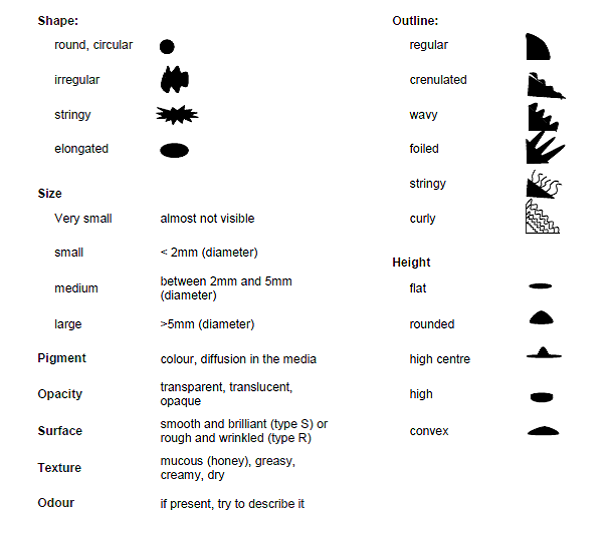
It is essential to confirm that isolates are representative, pure cultures and able to form nodules (or infect a host root system) on aseptically growing host plants, and thus satisfy Koch's postulates regarding causal organisms. Isolates must also be adequately preserved, evaluated and documented. Methods and criteria for this are described by Brockwell (1980), Date and Halliday (1987), FAO (1983), Moreira (2008) and Vincent (1970).

 

Future challenges/needs/gaps

Currently, the issues surrounding ownership of symbiotic bacteria and fungi are a nightmare. Private companies and even national collections have been working in the dark, and the final result is several references for the same strain of rhizobia or mycorrhiza. On the other hand, strains can be protected by specific patents, and according to the law, only the owners of the patents are legally allowed to use the strains. So far, for symbiotic bacteria and fungi, there are either no patents or they are not often patented. We believe that efforts are needed to clarify policies with regard to the collection and use of symbiotic bacteria so that poor farmers in developing countries will benefit.

The supply chain of symbiotic microbial inoculants, their cost at the national level and their availability and quality at the local level need improvement. For example, why are rhizobial inoculants not widely used in Africa by farmers producing legumes such as soybean, bean or groundnut? There is one well-known success story: in Zimbabwe, farmers producing soybean automatically use rhizobial inoculant. This is the result of huge efforts to convince farmers about the importance of systematically inoculating legumes with both rhizobia and mycorrhiza and of inoculating crops with mycorrhiza alone. This has been successful because the government set up a factory where qualified people started producing good-quality, affordable peat inoculum. By making it available to farmers, the technology has been well adopted. Even in recent years, during the economic downturn in Zimbabwe, most of the farmers have managed to purchase peat inoculum for their soybean production. Hence, efforts for improved production, quality control and access by farmers need to be improved so that collecting is done better and the symbiotic microbes are better conserved.

If there are improved benefits to be derived from a collection of symbiotic microorganisms, we need to identify the effective ones and see how to produce them on a large scale, in order to have good-quality inoculants available to farmers wherever they are.
We know that there are technical issues in the production of mycorrhizal inoculants, for example, but even then, some existing systems are performing well with several AMF species such as Glomus intraradices.

There needs to be a huge effort to fully exploit the high potential of microbes because they are still underutilized by poor end users. Interaction with the private sector seems to be the way forward in order to sustain the production of inoculants, but it requires industrial facilities with qualified people who know how to do it well. This sounds challenging but it is realistic because the market is huge and the demand is high. All that is needed is for everything to be organized and optimized.

 

Conclusions

• Sampling in the field needs to be correct in order to get representative soil samples corresponding to the existing indigenous symbiotic microbial communities.

• Storage of the samples (soils, roots, sporocarps, nodules) has to be done cautiously, and all this biological material requires immediate treatment, such as disinfection for nodules if the rhizobia contained therein need to be further isolated.

• Isolation of symbiotic bacteria and fungi is not very complicated but it has to be done in accordance with strict protocols; otherwise, the risk of isolating and cultivating contaminants is high. An example of this occurred some decades ago when different people were trying to isolate Frankia strains. They thought they were getting symbiotic strains of Frankia, but after inoculation to Casuarina seedlings, they did not get any nodules. Their stains were saprophytic Actinomyces, which is naturally present at the surface of the nodules, not symbiotic Frankia.

• While all these symbiotic microorganisms have to be tested under controlled conditions, they also have to be tested in the field in different agroecological zones. Then the effective inoculants have to be produced and provided to end users, which is the best way to justify collecting symbiotic microorganisms.

Back to list of chapters on collecting

 

References and further reading

Bagyaraj JD, Stümer SL. 2008. Arbuscular mycorrhizal fungi. In: Moreira FMS, Huising J, Bignell DE, editors. A Handbook of Tropical Soil Biology. Earthscan, London. pp.131–146.

Beaton G, Pegler DN, Young TWK. 1985. Gasteroid Basidiomycota of Victoria State, Australia: 8–9. Kew Bulletin 40:827–842.

Becking JH. 1977. Dinitrogen fixing associations in higher plants other than legumes. In: Hardy RWF, Silver W, editors. A Treatise on Dinitrogen Fixation. John Wiley & Sons, New York. pp.185–275.

Bontemps C, Elliott G, Simon MF, Does Reis Junior FB, Gross E, Lauton RC, Elias Neto N, Loureiro MF, de Faria S, Sprent J, James EK, Young P. 2010. Burkholderia species are ancient symbionts of legumes. Molecular Ecology 19:44–52.

Brockwell J. 1980. Experiments with crop and pasture legumes – principles and practice. In: Bergersen FJ, editor. Methods for Evaluating Biological Nitrogen Fixation. John Wiley & Sons, New York. pp.417–490.

Caldwell BE, Weber DF. 1970. Distribution of Rhizobium japonicum serogroups in soybean nodules as affected by planting dates. Agronomy Journal 62:12–14.

Chilvers GA, Pryor LD. 1965. The structure of eucalypt mycorrhizas. Australian Journal of Botany 13:245–259.

Cochran WG. 1977. Sampling Techniques. 3rd edition. John Wiley & Sons, New York.

Daniels BA, Skipper HD. 1982. Methods for the recovery and quantitative estimation of propagules from soil. In: Schenck NC, editor. Methods and Principles of Mycorrhizal Research. American Phytopathological Society, St. Paul, Minnesota. pp.29–35.

Date RA, Halliday J. 1987. Collecting, isolation, cultivation and maintenance of rhizobia. In: Elkan GH, editor. Symbiotic Nitrogen Fixation Technology. Marcel Dekker, New York. pp.1–27.

Date RA, Burt RL, Williams WT. 1979. Affinities between various Stylosanthes species as shown by rhizobial, soil pH and geographic relationships. AgroEcosystems 5:57–67.

Dedeurwaerdere T, Iglesias M, Weiland S, Halewood M. 2009. The use and exchange of microbial genetic resources for food and agriculture. Commission on Genetic Resources for Food and Agriculture. Background Study Paper No. 46. Food and Agriculture Organization of the United Nations, Rome. Available online (accessed 12 October 2011): ftp://ftp.fao.org/docrep/fao/meeting/017/ak566e.pdf.

Diem HG, Dommergues YR. 1983. The isolation of Frankia from nodules of Casuarina. Canadian Journal of Botany 61:2822–2825.

Dommergues YR, Duhoux E, Diem HG. 1998. Les arbres fixateurs d'azote. Editions speciales. CIRAD-FAO-IRD, Montpellier, France.

FAO. 1983. Technical Handbook on Symbiotic Nitrogen Fixation. Food and Agriculture Organization of the United Nations, Rome.

Gerdemann JW, Nicholson TH. 1963. Spores of mycorrhizal Endogene extracted from soil by wet sieving and decanting. Transactions of British Mycological Society 46:235–244.

Girlanda M, Perotto S, Bonfante P. 2007. Mycorrhizal fungi: their habitats and nutritional strategies. In: Kibicek CP, Druzhinina IS, editors. The Mycota: A Comprehensive Treatise on Fungi as Experimental Systems for Basic and Applied Research. Springer-Verlag, Berlin. pp.229–256.

Grand LF, Harvey AE. 1982. Quantitative measurement of ectomycorrhizae on plant roots. In: Schenck NC, editor. Methods and Principles of Mycorrhizal Research. American Phytopathological Society, St. Paul, Minnesota. pp.157–164.

Gregoire TG, Valentine HT. 2007. Sampling Strategies for Natural Resources and the Environment. Chapman and Hall/CRC Press, London.

Habte M. 2006. The roles of arbuscular mycorrhizas in plant and soil health. In: Ball AS, Fernandes E, Herren H, Husson O, Laing M, Palm C, Pretty J, Sanchez P, Sanginga N, Thies J, editors. Biological Approaches to Sustainable Soil Systems. CRC Press, Boca Raton, Florida. pp.129–147.

Hayman DS. 1982. Practical aspects of vesicular-arbuscular mycorrhiza. In: Subba Rao NS, editor. Advances in Agricultural Microbiology. Butterworths, London. pp.325–373.

Huising J, Coe R, Cares J, Louzada JN, Zanetti R, Moreira FMS, Susilo FX, Konate S, van Noordwijk M, Huang SP. 2008. Sampling strategy and design to evaluate below-ground biodiversity. In: Moreira FMS, Huising J, Bignell DE, editors. A Handbook of Tropical Soil Biology. Earthscan, London. pp.17–42.

Molina R, Palmer JG. 1982. Isolation, maintenance and pure culture manipulation of ectomycorrhizal fungi. In: Schenck NC, editor. Methods and Principles of Mycorrhizal Research. American Phytopathological Society, St. Paul, Minnesota. pp.115–129.

Molina R, Trappe JM. 1982. Applied aspects of ectomycorrhizae. In: Subba Rao NS, editor. Advances in Agricultural Microbiology. Butterworths, London. pp.305–424.

Moreira FMS. 2008. Nitrogen-fixing leguminosae-nodulating bacteria. In: Moreira FMS, Huising J, Bignell DE, editors. A Handbook of Tropical Soil Biology. Earthscan, London. pp.107–128.

Singleton PW, Somasegaran P, Nakao P, Keyser HH, Hoben HJ, Ferguson PI. 1990. Applied BNF Technologies: A Practical Guide for Extension Specialists. NifTAL, University of Hawaii, Honolulu.

Somasegaran P, Hoben HJ. 1985. Methods in Legume-Rhizobium Technology. NifTAL, University of Hawaii, Honolulu. Available online (accessed 10 October 2011): www.ctahr.hawaii.edu/bnf/Downloads/Training/Rhizobium%20technology/Title%20Page.PDF.

Sprent JI. 2009. Legume Nodulation: A Global Perspective. Wiley-Blackwell, Oxford, UK.

Stowers MD. 1987. Collection, isolation, cultivation and maintenance of Frankia. In: Elkan GH, editor. Symbiotic Nitrogen Fixation Technology. Marcel Dekker, New York. pp.29–53.

Varma A. 2008. Mycorrhiza. Springer-Verlag, Berlin.

Velasquez E, Garcia-Fraile P, Ramirez-Bahena MH, Rivas P, Martinez-Molina E. 2010. Bacteria involved in nitrogen-fixing legume symbiosis: current taxonomic perspective. In: Kan MS, Zaidi A, Musarrat J, editors. Microbes for Legume Improvement. Springer-Verlag, Vienna. pp.1–25.

Vincent JM. 1970. A Manual for the Practical Study of Root-Nodule Bacteria. Blackwell Scientific Publications, Oxford, UK.

Weber DF, Miller VL. 1972. Effect of soil temperature on Rhizobium japonicum serogroup distribution in soybeans. Agronomy Journal 64:796–798.

Wong CC, Sundram J, Date RA, Rougbley RJ. 1989. Nodulation of Leucaena leucocephala in acid soils of peninsular Malaysia. Tropical Grasslands 23:171–178.

 

Annex 1: Internet resources on collections of microbial cultures

The most comprehensive source of information on culture collections was published in 1972 by the World Data Center for Microorganisms (WDCM) (www.wfcc.info/wdcmdb). This is now the responsibility of the World Federation for Culture Collections (WFCC), which published the fourth edition of the World Directory of Collections of Cultures of Microorganisms in 1993 (Sugawara et al. 1993). This edition of the World Directory lists 481 culture collections, including services in 51 countries and the names of 334,312 strains of bacteria and 351,263 strains of fungi and yeasts. Information is indexed by geography, categories of holdings, main subjects and services like distribution, deposit, classification, identification, consultation and training, and personnel.

Formed under the umbrella of the International Union of Biological Sciences (IUBS) and a federation within the International Union of Microbiological Societies (IUMS), the WFCC is the main international body coordinating the activities of culture collections around the world. Its aim is to promote and support the establishment of culture collections and related services; to provide liaison and to set up information networks between the collections and their users; to organize workshops and conferences, publications and newsletters; and to work to ensure the long-term perpetuation of important collections.

In the last few years, computerized databases have been established in many service and research culture collections worldwide. Some of these are publicly accessible and have been collected by the WDCM, which, as of October 2011, maintained online data on 592 culture collections in 68 countries, comprising the following:

• microbials: 1,754,290

• bacteria: 768,608

• fungi: 507,792

• viruses: 19,148

• cell lines: 7,349

The WDCM database includes Culture Collections Information (CCINFO), with a search facility that allows searches by collection name and by strain, and a network of international and national federations and organizations, such as the European Culture Collections’ Organisation (ECCO) (www.eccosite.org), the Japanese Society for Culture Collections (JSCC) (www.nbrc.nite.go.jp/jscc/idb/search) database and the UK Federation for Culture Collections (UKFCC) (www.ukfcc.org).

Primary online and authoritative sources of information on collections of microbiological specimens

World Federation of Culture Collections (WFCC): www.wfcc.info/home
World Data Center for Microorganisms (WDCM): www.wfcc.info/wdcmdb
Culture Collections Information (CCINFO/collections): http://new.wfcc.info/ccinfo/collection
Culture Collections Information (CCINFO/strain),: www.wfcc.info/ccinfo/search/strain_search
World Federation of Culture Collections (WFCC/networks): www.wfcc.info/index.php/collections/networks

United Kingdom National Culture Collection (UKNCC): www.ukncc.co.uk

• Established to coordinate the activities of the UK national service collections of microbial organisms.

• Member collections offer a culture/cell supply service.

• Collection consists of actinomycetes, algae, animal cells, bacteria, cyanobacteria, filamentous fungi, nematodes, protozoa, mycoplasma, viruses and yeasts.

European Consortium of Microbial Resources Centres (EMbaRC): www.embarc.eu/project.html

• Aims to improve, coordinate and validate microbial resource centre delivery to European and international researchers from both public and private sectors.

References

Çaktu K, Turkoglu EA. 2011. Microbial culture collections: the essential resources for life. G.U. Journal of Science 24(2):175–180.

Dedeurwaerdere T, Iglesias M, Weiland S, Halewood M. 2009. The Use and Exchange of Microbial Genetic Resources for Food and Agriculture. Background Study Paper No. 46. Food and Agriculture Organization of the United Nations, Rome. Available on-line (accessed 13 October 2011): ftp://ftp.fao.org/docrep/fao/meeting/017/ak566e.pdf.

Krichevsky MI, Ross E, McManus C, Kirsop B. 1991. The microbial strain data network. Sydowia 43:123–134. Available on-line (accessed 13 October 2011): www.landesmuseum.at/pdf_frei_remote/Sydowia_43_0123-0134.pdf.

National Research Council. 1993. Managing Global Genetic Resources: Agricultural Crop Issues and Policies. National Academy Press, Washington DC.

Sugawara H, Ma J, Miyazaki S, Shimura J, Takishima Y. 1993. World Directory of Collections of Cultures of Microorganisms: Bacteria, Fungi and Yeasts. 4th edition. World Federation for Culture Collections, World Data Centre on Microorganisms. Wako-shi, Saitama, Japan.

 

Back to top

Chapter 7: Classifications of infraspecific variation in crop plants

K. Hammer
University of Kassel, Agrobiodiversity, Witzenhausen, Germany
E-mail: khammer.gat(at)t-online.de
Y. Morimoto
Bioversity International, Regional Office for Sub-Saharan Africa, Nairobi, Kenya
E-mail: y.morimoto(at)cgiar.org

	2011 version (0.5 MB)	1995 version (0.1 MB)
	Open the full chapter in PDF format by clicking on the icon above.

This chapter is a synthesis of new knowledge, procedures, best practices and references for collecting plant diversity since the publication of the 1995 volume Collecting Plant Diversity; Technical Guidelines, edited by Luigi Guarino, V. Ramanatha Rao and Robert Reid, and published by CAB International on behalf of the International Plant Genetic Resources Institute (IPGRI) (now Bioversity International), the Food and Agriculture Organization of the United Nations (FAO), the World Conservation Union (IUCN) and the United Nations Environment Programme (UNEP). The original text for Chapter 7: Classifications of Intraspecific Variation in Crop Plants, authored by P. Hanelt and K. Hammer, has been made available online courtesy of CABI. The 2011 update of the Technical Guidelines, edited by L. Guarino, V. Ramanatha Rao and E. Goldberg, has been made available courtesy of Bioversity International.

Please send any comments on this chapter using the Comments feature at the bottom of this page. If you wish to contribute new content or references on the subject please do so here.

Back to list of chapters on collecting

References for this chapter

Internet resources for this chapter

 

	Considerable intra-specific morphological variation in bottle gourd (Lagenaria siceraria) can be seen in fruit and seed size, shape, degree of development of the handle and shell thickness. The species was possibly the earliest crop to be domesticated by humans for use as a container that is light yet strong. (Photo: Y. Morimoto/Bioversity International)

Abstract

Infraspecific classifications are discussed as useful tools for the plant collector. Whereas formerly many different types of such classifications have been proposed and used, today we have relatively few modern examples. The reasons for this are discussed. In light of the general development in biodiversity, we should expect classification to take on greater importance, which would correspond to the often demanded increase in the importance of taxonomy.

 

Introduction

Germplasm collectors must be thoroughly familiar with what is known about the variation present within their target taxa if they are to sample them efficiently. In crops, this variation can be many times greater than in wild plants, especially for species that were domesticated early and have been widely spread around the world. Such variation is the result of both natural and artificial selection pressures. The latter may be conscious or unconscious and result from the application of diverse agricultural practices and from the disparate and changing demands of growers for specific agronomic and other properties. Variation may be in morphological, anatomical, karyological, ecological, physiological, biochemical and molecular characteristics. Explanatory surveys of genetic diversity can be useful preliminaries to germplasm collecting (von Bothmer and Seberg 1995). Most relevant for the collector in the field, however, is variation in morphological traits and ecological adaptation. Making use of a scheme for the classification of the morphological traits can help collectors to keep track of what they find and to compare the diversity of different areas (Moss and Guarino 1995).

The term “infraspecific” is used here to refer to variation within a cultivated taxon, but it should be pointed out that the crop in a wild-weedy-crop complex is often given subspecific rank, following the proposal of Harlan and De Wet (1971). Morphological infraspecific variation has been studied in many crops, though often for only a limited part of their geographic range or for a restricted set of characters. Formerly there were regular literature reviews on the taxonomy of cultivated plants, but these tasks have been taken over by the Plant Genetic Resources Abstracts (see Dearing and Guarino 1995).Traditional Floras sometimes consider variation within crop plants, though never in much detail. However, there are also specialized Floras dealing only with cultivated plants (see below). A recent encyclopaedia on cultivated plants (excluding ornamentals and forest trees), which also discusses the taxonomic framework of crop taxonomy and evolution, is provided by Hanelt and IPK (2001).

There is general agreement about the necessity and importance of such studies in cultivated plants (Andrews et al. 1999; Baum 1981; Diederichsen 2004; Hanelt 1988, 2001; Hetterscheid et al. 1996; Knüpffer and Ochsmann 2003; Mansfeld 1953; Ochsmann 2004; Styles 1986) in both applied and theoretical applications, ranging from the investigation of the history of domestication of plants and their subsequent evolution to the characterization of germplasm. However, the procedures used to develop the classifications and the resulting schemes themselves are extremely diverse, and a generally agreed-upon approach has not yet emerged (Hanelt 2001). Two extreme types of schemes may be recognized:

• complex hierarchical taxonomic subdivisions of a cultivated plant taxon, with many infraspecific taxa at several taxonomic ranks between the species and cultivar level (e.g., Dorofeev and Korovina 1979; Nechanský and Jirásek 1967)

• relatively simple, non-structured, special-purpose schemes with a few main groups (e.g., De Wet 1978) (The proposed culton concept [Hetterscheid and Brandenburg 1995] can be considered as a special-purpose scheme.)

Because selfing results in the variation within a crop being split into distinct homozygous lines, autogamous species tend to be relatively easier to classify in detail into many groups than allogamous species. In the past, this has led to over-splitting, a trend that has been somewhat reversed by genetic studies.

The different methods of approaching the infraspecific taxonomy of crops are discussed in this chapter insofar as they may be relevant to the needs of collectors. For further details, see Hanelt (1986) and Hanelt et al. (1993). Many classification proposals are written in languages other than English, but these somewhat overlooked approaches are also included in the focus of this paper.

 

Classifications

A classification scheme for classifying the infraspecific variation of crop plants has been proposed by Hanelt (1986; see also the 1995 version of this chapter):

1. Formal taxonomic classifications under the International Code of Botanical Nomenclature (ICBN) (http://ibot.sav.sk/icbn/main.htm):

a) Diagnostic-morphological
b) Phenetic-numerical
c) Ecogeographic

2. Informal classifications:

a) Diagnostic-morphological
b) Phenetic-numerical
c) Genetic

3. Mixed classifications

Two principle types of approaches are distinguished: formal taxonomic and informal classifications. Whereas in the former, formally recognized categories are used (more or less) according to the rules of the ICBN (McNeill et al. 2006), informal classifications use non-standard categories or categories as proposed in the International Code of Nomenclature of Cultivated Plants (ICNCP) (www.ishs.org/sci/icracpco.htm) (Brickell et al. 2009). In informal classifications, therefore, problems with nomenclature that result from the use of the ICBN are avoided, although there are other formal preconditions deriving from the ICNCP. Moreover, the two codes are not always compatible (Brandenburg and Schneider 1988; Ochsmann 2004) and a broadly accepted designation of a group is not guaranteed in informal classifications; therefore, communication of information on the material under study is more difficult.

Formal taxonomic classifications under ICBN

Diagnostic morphological classifications

Usually these classifications are based on a few, easily recognizable morphological characteristics and allow a rapid overview of variation within a crop. Several major publication projects have been based on this type of infraspecific classification, e.g., the Flora of Cultivated Plants of the Soviet Union (Dorofeev and Korovina 1979) and the Cultivated Plants of Hungary (Máthé and Priszter 1982). R. Mansfeld, the founder of the Gatersleben school of taxonomy, which has studied the infraspecific classification of several important cereal, legume and vegetable crops, provides a typical example with his morphological system of Triticum aestivum (Mansfeld 1951). He considers 12 characteristics and organizes infraspecific variation into more than 400 varieties, each differing from related ones in only one character. Mansfeld’s (1950) scheme for Hordeum vulgare can serve as another example. Below the species level, he applied the category of “convariety” (as defined by Alefeld 1866; see also Helm 1964) and accepted five convarieties, defined by major spike characters: convar. vulgare (convar. hexastichon), convar. intermedium, convar. distichon, convar. deficiens and convar. labile. Formerly, some of these convarieties were even described as separate species (not least, by Linnaeus). There are some differences in geographic distribution and even some crossing barriers among them, which might indicate that this category has some biological significance. “Varieties”, of which 191 are described, are purely artificial entities, however. In fact, such classifications are, as a rule, rather artificial, especially at lower taxonomic levels.

The same principles have been applied to Papaver somniferum. Based on the classification of Danert (1958), Hammer (1981) developed a system containing three subspecies: ssp. setigerum is the wild ancestor; ssp. somniferum and ssp. songaricum are both cultivated. The cultivated subspecies differ in having sulcate lobes of the stigmatic disc with dentate margins versus flat lobes with entire margins. These characters have been considered as important by some Papaver taxonomists and also show clear geographic differentiation. The convariety level is defined by indehiscent versus dehiscent capsules, another important character indicating different stages of domestication (Hanelt and Hammer 1987). The variety level is based on seed colour (resulting from selection pressures under domestication) and other characteristics. This system was recently rejected (Dittbrenner 2009; Dittbrenner et al. 2008), mainly using arguments from the culton-concept (Hetterscheid and Brandenburg 1995). After this, the Gatersleben genebank started to follow the Western approach in respect to infraspecific classifications.

Diagnostic-morphological classifications have proven to be very useful for keeping and elaborating large collections of cultivated plants (e.g., in genebanks), as well as for to the plant collector. Since the morphological entities that define these classifications can be recognized relatively easily, they can be used as the basis of field checklists. Rapid comparison of different areas with regard to the variation found there is possible and gaps in collections can be identified. Assessments of variation at different times based on such classifications have been used to estimate genetic erosion, for example in Sicily (Perrino and Hammer 1983; Prestianni 1926) and other parts of Italy (Hammer and Laghetti 2005).

The controversy between the proponents of diagnostic-morphological classification is yet to be resolved. It can best be demonstrated in wheat: Dorofeev and Korovina (1979) subdivide Triticum aestivum into two subspecies, three convarieties and 194 varieties. And whereas Mansfeld (1951) included T. compactum in T. aestivum, Dorofeev and Korovina classified it as a separate species with three convarieties and an additional 93 varieties.

While many interesting conclusions can be drawn on the basis of this system, as recently demonstrated by Filatenko et al. (2010), geneticists and plant breeders like Mac Key (1988), however, resist any further detailed subdivision between the levels of subspecies and cultivar. They do not see the necessity to describe entities that are not genetically meaningful, are characterized by a few common monofactorially inherited character states, and do not indicate properties that are important for the plant breeder (Hanelt 1988). Breeders are inclined to use more open, less formalized classifications, into which their material can be incorporated without difficulty (i.e., in the sense of the ICNCP) (Brickell et al. 2009). The polemics against diagnostic classifications have a long-standing history. Hawkes (1980) observed an East-West division with regard to the preference of such detailed diagnostic classifications (see also Hanelt 1988). Large collections of cultivated plants have been created in the eastern parts of Europe, for which diagnostic classifications have proved to be useful. Some exceptions are Percival (1921) and Mansfeld (1951), but they had considerably large collections at their disposal. At any rate, Mac Key’s (1966) system does not have detailed infraspecific treatment. A tool for the mutual understanding and use of both systems is now available (Hammer et al. 2011). But for the international use of Dorofeev and Korovina’s (1979) Russian wheat monograph, an English translation is necessary; there is one in preparation (Knüpffer et al. 2004).

In some cases, the classifications are of restricted applicability because they deal with the cultivated flora of a rather restricted area (e.g., Máthé and Priszter 1982). However, even country Floras of cultivated flora may employ a comprehensive concept of taxa, even allowing them to be used for a worldwide survey. The Flora of the Cultivated Plants of the Soviet Union is perhaps the best example. Some important contributions, in addition to the Triticum volume mentioned above, are Fursa and Filov (1982), Girenko and Korovina (1988), Kazakova (1978), Kobyljanskij (1989), Kobyljanskij and Lukjanova (1990), Kobyljanskij and Soldatov (1994), Makaševa (1979), Mukhina and Stankevič (1993), Pyženkov (1994), Šmaraev and Korovina (1982), Stankevič and Rep’ev (1999). In the last few years no new infraspecific classifications have appeared in this series. A recent monograph from the Vavilov Institute (Loskutov 2007), but not in the series cited above, has appeared without a detailed infraspecific treatment (which can be found in Kobyljanskij and Soldatov 1994). This could possibly be seen as a new trend.

The old morphological classifications of the Gatersleben school are listed by Hammer (1981). In addition to the species already mentioned, there are treatments of Beta vulgaris, Brassica oleracea, Glycine max, Linum usitatissimum, Lycopersicon esculentum, Nicotiana rustica, N. tabacum, Pisum sativum and many other crops. More recent treatments include Raphanus (Pistrick 1987), Brassica oleracea (Gladis and Hammer 2003), Brassica spp. (Gladis and Hammer 1992), Coriandrum (Diederichsen and Hammer 2003) and Ocimum (Eckelmann 2003). For a recent compilation of diagnostic-morphological classifications, see Landsrath and Hammer (2007).

Obviously, there has been a certain decline in the last few years. A potential problem with diagnostic-morphological classifications is still the difficulty in comprehension and their limited availability – many are not available in English and might be difficult to obtain. As a result, some older classifications, such as that of Percival (1921) on Triticum, are sometimes used even today. The forthcoming edition of Dorofeev and Korovina (1979) in English could improve the situation, at least with respect to Triticum.

Most of the available diagnostic morphological classifications for Central European crop plants are, as already mentioned, included in a modern treatment of Alefeld’s “Agricultural Flora” (Landsrath and Hammer 2007). Alefeld and Körnicke (Hammer 2005) can be considered as the founders of intensive work with those classifications.

Phenetic-numerical classifications

These classifications consider a large number of characters. Various multivariate mathematical methods are used to calculate similarities among infraspecific taxa and to identify groupings. There are several examples (reviewed by Schultze-Motel 1987; see also Baum et al. 1984) but none is particularly convincing in the context of formal taxonomy. They cannot be recommended for the practical use of the plant collector.

Ecogeographic classifications

Such classifications have been developed by the Vavilov Institute, based on the hypothesis that, in an area where selection pressure from environmental factors, cultivation practices, propagation methods, etc., is relatively homogeneous, a crop will tend to have a certain genetic integrity (Vavilov 1940). An example of ecogeographic classification is that proposed by Flaksberger (1935) for Triticum aestivum, which includes two subspecies, 15 proles and six subproles.

New taxonomic categories have often been introduced. Groups are largely defined by their geographic origin and by characteristics that reflect the agricultural and ecological conditions to which they are adapted (e.g., reproductive phenology, pest and disease resistance, growth characteristics, etc.). In general, field experiments are necessary to verify the categories and to incorporate new accessions into such a classification. Therefore, a collector might not be able to apply them directly during fieldwork. However, they might be very useful for the characterization of collections, facilitating the use of the material by breeders. There is still no bridge between formal ecogeographical classifications and the use of an ecogeographic approach in fieldwork (Maxted et al. 1995).

Informal taxonomic classifications

Diagnostic-morphological classifications

There are some regional studies of this type. The classification of French bush bean cultivars is one. They have been arranged into three categories: groups, sections and classes (Anon. 1983). Pod characteristics (11 character states) are used to differentiate groups and sections; and leaf colour, pod length, colour of unripe pods and length of bracts (12 character states) for differentiating classes. The resulting system comprises five groups, 14 sections and many classes. Another example, also from Phaseolus vulgaris, shows that the input of biochemical methods (in this case, phaseoline types) can lead to phytogenetically more relevant groupings within an informal diagnostic-morphological classification (Krell and Hammer 2008, Singh et al. 1991).

The extremely reduced possibilities for infraspecific classifications of cultivated plants under the ICNCP (Brickell et al. 2009), largely following the proposal of the culton concept (Hetterscheid and Brandenburg 1995), which is still heavily disputed (Hanelt 2001, Pickersgill and Karamura 1999), have to be considered here. Many new approaches are of this type, e.g., in Cruciferae, Cucurbitaceae and also Gramineae. They are formally dependent on the ICNCP and thus they lack the flexibility of informal classifications. This is one of the disadvantages of this code, which became user driven (by the flower and seed industry) under the forceful argumentation of the cultonomists.

Phenetic-numerical classifications

One of the best examples of this type of classification is the study of the South American cultivars of cassava (Manihot esculenta) by Rogers and Fleming (1973). They used 55 character states and defined 19 groups of cultivars. Within these groups, there is a high degree of phenotypic similarity, and evidently also considerable genetic similarity. New material can be easily incorporated into the proposed classification scheme; however, the evaluation of the basic data for this type of study is very time consuming.

The range of potentially relevant morphological characteristics for a species, which can be measured in morphological analysis, is summarized in descriptor lists. Some of the crop descriptors and monographs have been published and are available online on the Bioversity International website (www.bioversityinternational.org/publications.html).

Genetic classifications

This type of classification is only possible in crops with well-studied genetics, such as Pisum sativum (Blixt 1979), where the genes responsible for the expression of many different characteristics are known. In peas, there has also been an attempt to combine a formal diagnostic and a genetic classification (Lehmann and Blixt 1984). It is difficult to incorporate new material into such classifications. Test crosses are necessary and multifactoral characteristics cannot be included at all.

Classifications based on genomic composition are somewhat different. An example is that of Simmonds for the edible fruit-bearing bananas (Simmonds 1966; Simmonds and Weatherup 1990). These are classified by references to ploidy (2×, 3×, 4×) and the genomic contribution made by two diploid wild species (AA Musa acuminata and BB Musa balbisiana). Some 15 characteristics are used to distinguish among cultivar groups. Infraspecific items are not involved in this example. Problems with species designations (and also with infraspecific ones) arise when dealing with hybrid genera, as, e.g., × Triticosecale, according to the ICBN (Hammer et al. 2011).

In the last decade, increased attention has been devoted to molecular marker technologies, including DNA sequences. These have provided a wealth of data, which, together with phenotypic and ecological data, have significantly increased our understanding of the intra-specific dynamics of these genetic resources. The study findings provide not only information for classification but also a geographic framework of references to elucidate patterns of genetic diversity and domestication, constituting a source of diversity for a wide range of traits (Gepts et al. 1999). Combined with phenotypic data and multivariate statistical analysis, the recent progress in molecular mapping also provides opportunities to identify and transfer genes (geneflow) for quantitative traits and processes of domestication (Tanksely and McCouch 1997). Molecular marker technologies are useful tools for measuring lineages and comparative relationships between individuals, populations and species, obtaining evidence of recent bottlenecks in populations in size, as well as documenting geneflow, recombination and seed supply and identifying varieties (Brown et al. 1996).

In the genus Vigna, family of Fabaceae, for instance, Tomooka et al. (2002) described the subgenus of Vigna ceratotropis and suggested revising the nomenclature of the group, based on past taxonomic treatments and their biosystematics results, including diversity distributions, species relationships and cross-compatibility studies. Saravanakumar et al. (2004) conducted a random amplified polymorphic DNA (RAPD) analysis to enhance understanding of the diversity of Vigna species from Palney Hills in India, to determine (1) the taxonomic relationship between V. trinervia var. trinervia and V. trinervia var. bourneae, (2) the distinction between V. trinervia collected at a high altitude of about 1000m and at a low altitude, (3) the relationship among V. radiate var. sublobata from different geographic locations and (4) relationships between V. dalzelliana and other species.

In the genus Oryza, the taxonomy of the three diploid CC genome of Oryza species (O. eichingeri, O. officinalis and O. rhizomatis) has been confused and several different names have been used in the literature and herbaria (e.g., Dally and Second 1990; Duistermaat 1987; Harriman 1994; Katayama and Ogawa 1974; Sharma and Shastry 1965; Tateoka and Pancho 1963). This was because two major useful characteristics (chromosome number and rhizome formation) are not readily visible for some species in the complex. Later molecular-based diversity studies helped to find the relationships within the diploid CC genome species complex, thus showing their evolutionally history (e.g., AFLP: Aggarwal et al. 1999; isozymes: Second 1984; RFLP: Wang et al. 1992; ISSR: Joshi et al. 2000; chloroplast SSR: Ishii and McCouch 2000; 5SDNA sequences: McIntyre et al. 1992; RAPDs Xie et al. 1998).

In the common bean, genus Phaseolus, Debouck (1999) has indicated generic limitations in the taxonomic classification. He comments that over 400 species of Phaseolus have been named over the past two centuries, often with poor description or lacking good type specimens. He also indicates that “we do not know yet exactly how many Phaseolus species are existing, 50–60 species would be a reasonable estimate” on the basis of species cross-compatibility, several molecular marker studies (Fofana et al. 1997, 1999; Jaaska 1996; Jacob et al. 1995) and extensive herbarium field exploration surveys, including his own (Debouck 1991, 1999).

Gepts et al. (1999) look at the genetic diversity and domestication of the common bean (Phaseolus vulgaris). For the faba bean (Vicia faba L.), RAPD and restriction fragment length polymorphism (RFLP) techniques were employed to analyse the same faba bean populations described by Muratova (1931), to find possible relationships within the V. faba genepool from different geographic regions and to try to elucidate the routes of dispersal of the faba bean as a crop (Potokina et al. 1999).

Most recently, molecular classification techniques have grown in importance to crop improvement. Arai-Kichise et al. (2011) used single nucleotide polymorphisms (SNPs) and insertions-deletions (InDels) between highly homologous genomes, and performed whole-genome sequencing of a landrace of japonica rice. They identified 132,462 SNPs between the genomes of Omachi and Nipponbare, which are closely related cultivars. They also validated InDels on a part of chromosome 2 as DNA markers and successfully genotyped five japonica rice cultivars. This provides a methodology and extensive data on SNPs and InDels available for whole-genome genotyping and marker-assisted breeding.

However, these techniques have been applied so far mostly to “model species” such as humans, yeasts and some of the major crops such as rice, maize and wheat, as well as beans. The technology is still expensive, and a positive return on investment in this technology has not yet been recognized.

Nevertheless, classifications based on genetic data (including molecular markers) are probably the best guides for germplasm collectors when collecting plant genetic resources – better than mostly morphological/botanical traits. Since the genetics of a species need to be well understood for this, the value of such genetic analyses is greater for collectors when gap-filling collections are made.

Mixed classifications

There is no single classification approach suitable for all possible demands; different aims can be achieved with different types of classifications. Hanelt (1972) proposed a combination of classifications for Vicia faba: a formal diagnostic classification into two subspecies, three varieties and six subvarieties (based mainly on seed size, form and structure of pods) was combined with an informal classification into 14 races, based mainly on ecogeographic data. A similar approach has been used for Citrullus lanatus (Fursa 1981).

In a number of cases, Jeffrey (e.g., in the “Compositae” [Jeffrey 2001]) preferred the informal classification according to the ICNCP (open classification, according to Brandenburg 1999). For Cynara cardunculus, Jeffrey considers a cardoon group and a globe artichoke group, with broad synonymy from the formal classifications (closed classification, according to Brandenburg 1999). This can be considered as an extreme case of a mixed classification. Hammer (2001), in treating the Chenopodiaceae, classified Beta according to a formal system and provided the informal groups after the synonymy, e.g., sugar beet: Beta vulgaris var. altissima (the sugar beet group).

At any rate, with the new development of the ICNCP, more synonymy-like indications will be necessary for exact agrobotanical work, especially in the group of cultivated plants within Mansfeld’s definition (Hanelt and IPK 2001).

	Landraces are named according to specific morphological characteristics of the fruit, or sometimes after the village where they were obtained. This homestead is at “Mutha” village in Kitui District, Kenya, where local people classified 242 gourds into 33 landraces. (Photo: Y. Morimoto/Bioversity International)
	Diversity in uses - associated with diverse fruit traits - is the most important driving force for strong selection. Farmers carefully choose several different types from their previous harvest depending on their needs. Varieties used for oil (right) have distinctly larger seeds than varieties used for containers and food (left row). (Photo: Y. Morimoto/Bioversity International)

Farmers’ classifications

Farmers’ classification is considered to be the most uncertain classification system; however, it is the most useful guide in narrowing the range of agro-morphological criteria, which are usually linked to the genetic diversity of a crop. They are used by farmers to distinguish and name crop varieties and are commonly the basis for farmers’ selection of varieties, which is important in shaping the population over time (Jarvis et al. 2000). It is therefore of direct relevance to farmers and plant breeders in their use of germplasm. Berlin (1999) states that while folk or ethnobotanical classifications are not comprehensive, he gives an example of the naming behaviour of the Tzeltal Maya community in Chiapas, Mexico, which is to conceptually relate an unknown plant to a prototype that has been encountered before. Berlin refers to this as “exemplar comparison” (from Medin 1989) and describes it as the basis of the “perceptual affinities” of the new target species to the original prototype.

Many studies have pointed out how farmers recognize and name the crops they grow according to agromorphological, ecological-adaptive, quality and use characteristics (Bellon and Brush 1994; Boster 1985; Quiros et al. 1990; Schneider 1999; Soleri and Cleveland 2001; Teshome et al. 1997). The names of farmers’ varieties, for instance, are often related to the original source of the material, the morphology of the plant, agronomic performance, adaptation to particular environmental factors, and the use of the material, including its role in religious ceremonies. When collecting information from farmers, it is important to note down the exact name of each variety as given by the farmer, without modifying it, using the local alphabet if possible (Jarvis et al. 2000). However, farmers might not be consistent in naming and describing landraces. Studies have indicated that sometimes there is consistency between variety names and genetic distinctiveness (Karamura 2004; Mar and Holly 2000), but other times there is not. For example, a study in Ethiopia has shown different names for the same variety, reflecting an emphasis on different qualities by different farmers or communities. Another example is durum wheat in Ethiopia. In some villages, a variety is called “white”, whereas in the others, the same variety is called “early” (Tanto 2001). Tesfaye and Ludders (2003) found similar evidence in Ethiopia for enset, a clonally propagated crop, for which a few landraces assumed different names at different locations. Sawadogo et al. (2005) indicate that differences in variety names in the same village or community reflect differences in the languages used to name the variety. Farmers’ names also vary with the gender, age or ethnic group of the individual (Canh et al. 2003; Hue et al. 2003; Karamura et al. 2004; Mulumbo et al. 2004). Fujimoto (1997) mentions that farmers also categorize enset landraces based on their reminiscences, such as which offspring are derived from which mother plant, a classification he describes as “genealogical classification”. Sigeta (1995) indicates that farmers’ names are described differently depending on individual recognition. In order to enhance better understanding of this classification, he emphasizes that researchers need to focus more on farmers’ actions and recognition rather than the morphological characteristics and performance of the plants.

In addition to consistency in variety names, it is important to find different degrees of adaptive and quality traits and to develop a level of consensus between farmers on their selection criteria for planting seeds. The structure of genetic variability between and within farmer-named varieties has also been described using biochemical and molecular markers. Teshome et al. (1999) assessed farmers’ knowledge of the resistance of sorghum landraces to the rice weevil in storage and revealed that, according to biochemical and molecular markers, the level of landrace susceptibility to the weevil was highly correlated with farmers’ classifications.

These research approaches require intensive investigation with farmers, visits to the field and participatory measurement during all stages of crop development. Clarification of what constitutes a landrace at each level (individual, family, community, village and region) is the first step toward defining the amount and distribution of crop diversity maintained by farmers.

 

Conclusions

 It is well known that most of the more important and widespread crop species are characterized by an enormous amount of infraspecific variation. Familiarity with this is essential for the effective collecting of plant genetic resources. There are many publications on the infraspecific taxonomy of crop plants, but many have been written in languages other than English (particularly the most important papers of the Vavilov school).

A variety of methods have been proposed for the classification of crop plants. Those most appropriate for collectors seem to be the ones based on easily recognizable characteristics of gross morphology. Variation in such characteristics can be used to establish taxonomically formal or informal diagnostic classifications, which will be no less useful for the later management of collections than for the collector in the field.

As discussed here, there has been a reduction in the use of infraspecific classifications, which is connected with a reduction in knowledge about the functions and usefulness of such classifications. Infraspecific classifications are of limited use for plant breeding, but they are of great use to the plant collector and to genebank management. Together with a six-fold paradigm shift in the area of plant genetic resources (Hammer 2003), we are losing the methods and means that are helpful for their collection, maintenance and characterization. The abandonment of infraspecific classifications, which has been strongly advocated for many crops, leads to a loss of information (quantity and quality).

The momentum that has been lost depends on the crop, the kind of research being done and the research community. In barley, for example, infraspecific classification has been largely abandoned, whereas in wheat, many publications still use infraspecific classifications, especially when reporting about landraces. Moreover, recent developments in the Cultivated Plant Code (Brickell et al. 2009) and its application have exclusively concerned plants grown in developed countries, “with well-organised trades in harvested products, planting material or both, and often with International Registration Authorities to regulate the application of cultivar names” (Pickersgill and Karamura 1999). Landraces with their characteristic and rich morphological structure are today neglected in this respect by the Code.

Back to list of chapters on collecting

 

References and further reading

Aggarwal AK, Brar DS, Nandi S, Huang N, Khush GS. 1999. Phylogenetic relationships among Oryza species revealed by AFLP markers. Theoretical and Applied Genetics 98:1320–1328.

Alefeld F. 1866. Landwirthschaftliche Flora. Wiegandt & Hempel, Berlin.

Anon. 1983. Description et essai de classification de variétés de Haricot Nain. National Institute for Agricultural Research (INRA), Versailles.

Andrews S, Leslie AC, Alexander C, editors. 1999. Taxonomy of Cultivated Plants: Third International Symposium. Royal Botanic Gardens, Kew, UK.

Arai-Kichise Y, Shiwa Y, Nagasaki H, Ebana K, Yoshikawa H, Yano M, Wakasa K. 2011. Discovery of genome-wide DNA polymorphisms in a landrace cultivar of japonica rice by whole-genome sequencing. Plant Cell Physiology 52(2):274–282.

Baum BR. 1981 Taxonomy of the infraspecific variability of cultivated plants. Kulturpflanze 29:209–239.

Baum BR, Duncan T, Phillips RB. 1984. A bibliography of numerical phenetic studies in systematic botany. Annals of the Missouri Botanical Garden 71:1044–1060.

Bellon MR, Brush SB. 1994. Keepers of the maize in Chiapas, Mexico. Economic Botany 48:196û209.

Berlin B. 1999. Chapter 4: How a folk botanical system can be both natural and comprehensive: one Maya Indian’s view of the plant world. In: Medin DL, Atran S, editors. Folkbiology. Massachusetts Institute of Technology. pp.71–89.

Blixt S. 1979. Some genes of importance for the evolution of the pea in cultivation (and a short presentation of the Weibullsholm-PGA collection). In: Zeven AC, van Harten AM, editors. Broadening the Genetic Basis of Crops. PUDOC, Wageningen, The Netherlands. pp.195–202.

Boster JS. 1985. Selection for perceptual distinctiveness: evidence from Aguaruna cultivars of Manihot esculenta. Economic botany 39(3):310–325.

Brandenburg WA. 1999. Crop-weed complexes and the culton concept. In: Andrews S, Leslie AC, Alexander C, editors. Taxonomy of Cultivated Plants: Third International Symposium. Royal Botanic Gardens, Kew, UK. pp.145–157.

Brandenburg WA, Schneider F. 1988. Cultivar grouping in relation to the International Code of Nomenclature for Cultivated Plants. Taxon 37:141–147.

Brickell CD, Alexander C, David JC, Hetterscheid WLA, Leslie AC, Malecot V, Xiaobai Jin, Cubey JJ, editors. 2009. New Edition of the International Code of Nomenclature for Cultivated Plants. Scripta Horticulturae 10. International Society for Horticultural Science, Leuven, Belgium.

Brown SM, Hopkins MS, Mitchell SE, Wang TY, Kresovich S, Duncan RR, Senior ML and Gonzalez-Candelas F. 1996. Multiple methods for the identification of polymorphic simple sequence repeats (SSRs) in sorghum (Sorghum bicolor L. Moench). Theoretical and Applied Genetics 93:190–198.

Canh NT, On TV, Trung NV, Tiep CA, Lam HV. 2003. Preliminary study of genetic diversity in rice landraces in Ban Khoang Commune, Sa Pa District. In: Tuan HD, Hue NN, Sthapit BR, Jarvis DI, editors. On-Farm Management of Agricultural Biodiversity in Vietnam: Proceedings of a Symposium, 6–12 December 2001, Hanoi, Vietnam. International Plant Genetic Resources Institute, Rome. Available online (accessed 20 October 2011): www.bioversityinternational.org/index.php?id=19&user_bioversitypublications_pi1%5BshowUid%5D=2750.

Dally AM, Second G. 1990. Chloroplast DNA diversity in wild and cultivated species of rice (genus Oryza, section Oryza). Cladistic-mutation and genetic distance analysis. Theoretical and Applied Genetics 80:209–222.

Danert S. 1958 Zur Systematik von Papaver somniferum L. Kulturpflanze 6:61–88.

de Wet JMJ. 1978 Systematics and evolution of Sorghum sect. Sorghum (Gramineae). Amer. J. Bot. 65: 477 – 488.

Dearing JA, Guarino L. 1995 Bibliographic databases for plant germplasm collectors. In: Guarino L, Ramanatha Rao V, Reid R editors. Collecting Plant Genetic Diversity: Technical Guidelines. CAB International, Wallingford, UK. pp.229–254. Available online (accessed 20 October 2011): http://cropgenebank.sgrp.cgiar.org/images/file/procedures/collecting1995/Chapter13.pdf.

Debouck, DG. 1991. Systematics and morphology. In: Van Schoonhoven A, Voysest O, editors. Common Beans: Research for Crop Improvement. CAB International, Wallingford, UK. pp.55–118.

Debouck, DG. 1999. Diversity in Phaseolus species in relation to the common bean. In: Singh SP, editor. Common Bean Improvement in the Twenty-First Century. Kluwer Academic Publishers, Dordrecht, The Netherlands. pp.25–52.

Diederichsen A. 2004. Case studies for the use of infraspecific classification in managing germplasm collections in cultivated plants. Acta Horticulturae 634:127–139.

Diederichsen A, Hammer K. 2003. The infraspecific taxa of coriander (Coriandrum sativum L.). Genetic Resources and Crop Evolution 50:33–63.

Dittbrenner A. 2009. Morphologische, phytochemische und molekulare Untersuchungen zur infraspezifischen Diversität von Schafmohn (Papaver somniferum L.). Dissertation. Martin Luther University of Halle-Wittenberg, Germany.

Dittbrenner A, Lohwasser U, Mock H-P, Börner A. 2008. Molecular and phytochemical studies of Papaver somniferum in the context of infraspecific classification. Acta Horticulturae 799:81–88.

Dorofeev VF, Korovina ON, editors. 1979. Pšenica (Wheat). Kul’turnaja Flora. Vol. 1. Kolos, Leningrad.

Duistermaat H. 1987. A revision of Oryza (Gramineae) in Malesia and Australia. Blumea 32:157–193.

Eckelmann S. 2003. Biodiversität der Gattung Ocimum L., insbesondere der Kultursippen. Schriften zu Genetischen Ressourcen 19. Kassel, Bonn.

Filatenko AA, Hammer K, Al Khanjari S, Buerkert A. 2010. Six new botanical varieties of Triticum from Oman. Genetic Resources and Crop Evolution 57:1135–1139.

Flaksberger CA. 1935. Cereals: Wheat. In: Vulf EV, editor. Flora of Cultivated Plants. Vol. 1. State Agricultural Publishing Co., Moscow and Leningrad.

Fofana, B, Vekemans X, du Jardin P, Baudoin JP. 1997. Genetic diversity in Lima bean (Phaseolus lunatus L.) as revealed by RAPD markers. Euphytica 95:157–165.

Fofana B, Baudoin JP, Vekemans X, Debouck DG, du Jardin P. 1999. Molecular evidence for an Andean origin and a secondary gene pool for the Lima bean (Phaseolus lunatus L.) using chloroplast DNA. Theoretical and Applied Genetics 98:202–212.

Fujimoto T. 1997. Enset and its varieties among the Malo, south western Ethiopia. In: Fukui K, Kurimoto E, Shigeta M, editors. Ethiopia in Broader Perspective. Vol. III. Papers of the 13th International Conference of Ethiopian Studies, 12–17 December 1997, Kyoto. pp.867–882.

Fursa TB. 1981. Intraspecific classification of water-melon under cultivation. Kulturpflanze 29:297–300.

Fursa TB, Filov AI. 1982. Tykvennye [Cucurbitaceae – Citrullus, Cucurbita]. In: Brežnev DD, editor. Kul’turnaja Flora SSSR. Vol. 21. Kolos, Moscow.

Gepts P, Papa R, Coulibaly S, Gonzalez Mejia A, Pasquet R. 1999. Wild legume diversity and domestication - insights from molecular methods. In: The 7th MAFF International Workshop on Genetic Resources: Part 1. Wild Legumes. National Institute of Agrobiological Resources, Tukuba, Ibaraki, Japan. pp.19–31. Available online (accessed 20 October 2011): www.gene.affrc.go.jp/pdf/misc/international-WS_07.pdf.

Girenko MM, Korovina ON. 1988. Listovye ovoščnye rastenija [Leafy vegetables – asparagus, rhubarb, sorrel, spinach, purslane, garden cress, dill, chicory, lettuce]. In: Dorofeev VF, editor. Kul’turnaja Flora SSSR. Vol. 12. Agropromizdat, Leningrad.

Gladis Th, Hammer K. 1992. Die Gaterslebener Brassica-Kollektion – Brassica juncea, B. napus, B. nigra und B. rapa. Feddes Repertorium 103:469–507.

Gladis Th, Hammer K. 2003. Die Brassica-oleracea-Gruppe. Schriften VEN, Lennestadt, Germany.

Hammer K. 1981. Problems of Papaver somniferum classification and some remarks on recently collected European poppy land-races. Kultupflanze 29:287–296.

Hammer K. 2001. Chenopodiaceae. In: Hanelt P and IPK, editors. Mansfeld’s Encyclopedia of Agricultural and Horticultural Crops. Vol. 1. Springer, Berlin. pp.235–284.

Hammer K. 2003. A paradigm shift in the discipline of plant genetic resources. Genetic Resources and Crop Evolution 50:3–10.

Hammer K. 2005. Der Poppelsdorfer Forscher Friedrich August Körnicke (1828–1908). Vortr. Pflanzenzüchtg 67:7–11.

Hammer K, Laghetti G. 2005. Genetic erosion – examples from Italy. Genetic Resources and Crop Evolution 52:629–634.

Hammer K, Filatenko AA, Pistrick K. 2011. Taxonomic remarks on Triticum L. and ×Triticosecale Wittm. Genetic Resources and Crop Evolution 58(1):3–10.

Hanelt P. 1972. Die infraspezifische Variabilität von Vicia faba L.und ihre Gliederung. Kulturpflanze 20:75–128.

Hanelt P. 1986. Formal and informal classifications of the infraspecific variability of cultivated plants – advantages and limitations. In: Styles BT, editor. Infraspecific Classification of Wild and Cultivated Plants. Clarendon Press, Oxford, UK. pp.139–156.

Hanelt P. 1988. Taxonomy as a tool for studying plant genetic resources. Kulturpflanze 36:169–187.

Hanelt P. 2001. Preface. In: Hanelt P and IPK, editors. Mansfeld’s Encyclopedia of Agricultural and Horticultural Crops (Except Ornamentals). Vol. 1. Springer, Berlin. pp.xxv–xxvii.

Hanelt P, Hammer K. 1987. Einige infragenerische Umkombinationen und Neubeschreibungen bei Brassica L. und Papaver L. Feddes Repertorium 98:553–555.

Hanelt P and IPK, editors. 2001. Mansfeld’s Encyclopedia of Agricultural and Horticultural Crops. Springer, Berlin.

Hanelt P, Linne von Berg G, Klaas M. 1993. Taxonomische Untersuchungen zur infraspezifischen Variabilität bei Kulturpflanzen. Vortr. Planzenzüchtg 25:212–227.

Harlan R, de Wet JMJ. 1971. Towards a rational taxonomy of cultivated plants. Taxon 20:509–517.

Harriman NA. 1994. Poaceae. In: Dassanayake, MD, FR Fosberg, editors. A Revised Handbook to the Flora of Ceylon. Vol. 8. Amerind, New Dehli. Pp.326–330.

Hawkes JG. 1980. Biosystematic studies of cultivated plants as an aid to breeding research and plant breeding. Kulturpflanze 29:327–335.

Helm J. 1964. 100 Jahre Kulturpflanzentaxonomie. Dr. Friedrich Alefeld zum Gedächtnis. Kulturpflanze 12:75–92.

Hetterscheid WLA, Brandenburg WA. 1995. Culton versus taxon: conceptual issues in cultivated plants taxonomy. Taxon 44:161–175.

Hetterscheid WLA, van den Berg RG, Brandenburg WA. 1996. An annotated history of the principles of cultivated plant classification. Acta Botanica Neerlandica 45:123–134.

Hue N, Trinh L, Ha N, Sthapit B, Jarvis D. 2003. Taro cultivar diversity in three ecosites of North Vietnam. In: Tuan HD, Hue NN, Sthapit BR, Jarvis DI, editors. On-Farm Management of Agricultural Biodiversity in Vietnam. Proceedings of a symposium, 6–12 December 2001, Hanoi, Vietnam. International Plant Genetic Resources Institute, Rome. Available online (accessed 20 October 2011): www.bioversityinternational.org/fileadmin/bioversity/publications/pdfs/863.pdf.

Ishii T, McCouch SR. 2000. Microsatellites and microsynteny in the chloroplast genomes of Oryza and eight other Graminae species. Theoretical and Applied Genetics 100:1257–1266.

Jaaska, V. 1996. Isoenzyme diversity and phylogenetic affinities among the Phaseolus beans (Fabaceae). Plant Systematics and Evolution 200:233–252.

Jacob M, Zink D, Nagl W. 1995. RFLPs of the rRNA genes in the genus Phaseolus. Genetic Resources and Crop Evolution 42:97–106.

Jarvis DI, Myer H, Klemick L, Guarino L, Smale M, Brown AHD, Sadiki M, Sthapit B, Hodgkin T. 2000. Chapter 4. Agromorphological characters, farmer selection and maintenance. In: Jarvis DI, Myer H, Klemick L, Guarino L, Smale M, Brown AHD, Sadiki M, Sthapit B, Hodgkin T. A Training Guide for In Situ Conservation On-Farm. Version 1. International Plant Genetic Resources Institute, Rome. pp.49–70. Available online (accessed 20 October 2011): www.bioversityinternational.org/fileadmin/bioversity/publications/pdfs/611.pdf?.

Jeffrey C. 2001. Compositae (Asteraceae). In: Hanelt P. and IPK, editors. Mansfeld’s Encyclopedia of Agricultural and Horticultural Crops. Vol. 4. Springer, Berlin. pp.2035–2145.

Joshi SP, Gupta VS, Aggarwal RK, Ranjekar PK, Brar DS. 2000. Genetic diversity and phylogenetic relationship as revealed by inter simple sequence repeat (ISSR) polymorphism in the genus Oryza. Theoretical and Applied Genetics 100:1311–1320.

Karamura D. 2004. Estimation of distinct clones in the Uganda national banana germplasm collection. Presentation at a Workshop on Data Variables and Structure to Answer Questions That Support the Conservation and Use of Crop Genetic Diversity On-Farm, 20–24 September 2004, Rome.

Karamura D, Karamura E, Wasswa J, Kayiwa B, Kalanzi A, Nkwiine C. 2004. Analysis of community banana based management practices: A farmer’s perspective towards maintaining diversity. Presentation at a Workshop on Data Variables and Structure to Answer Questions That Support the Conservation and Use of Crop Genetic Diversity On-Farm, 20–24 September 2004, Rome.

Katayama T, Ogawa T. 1974. Cytological studies on the genus Oryza. VII. Cytogenetical studies on F1 hybrids between diploid O. punctata and diploid species having C genome. Japanese Journal. Breed 24:165–168.

Kazakova AA. 1978. Luk [Allium]. In: Brežnev DD, editor. Kul’turnaja Flora SSSR. Vol. 10. Kolos, Leningrad.
Knüpffer H, Ochsmann A. editors. 2003. Rudolf Mansfeld and Plant Genetic Resources. Schriften zu Genetischen Ressourcen 22. Kassel, Bonn.

Knüpffer H, Morrison LA, Filatenko AA, Hammer K, Morgounov A, Faberová I. 2004. English translation of the 1979 Russian taxonomic monograph of Triticum L. by Dorofeev et al.: Project progress report. Schriften zu Genetischen Ressourcen 22:282–283.

Kobljanskij VD, editor. 1989. Rož [Rye]. In: Dorofeev VF, editor. Kul’turnaja Flora SSSR. Vol. 2, part 2. Agropromizdat, Leningrad.

Kobyljanskij VD, Lukjanova MV, editors. 1990. Jačmen [Barley]. In: Krivčenko VI, editor. Kul’turnaja Flora SSSR. Vol. 2, part 1. Agropromizdat, Leningrad.

Kobyljanskij VD, Soldatov VN, editors. 1994. Oves [Oat]. In Kul’turnaja Flora. Vol. 2, part 3. Kolos, Moscow.

Krell K, Hammer K. 2008. Five hundred years of garden bean (Phaseolus vulgaris L.) in Europe. Botany, history of introduction and genetic resources. Schriften VEN 7. Cremlingen – Schandelah.

Landsrath S, Hammer K. 2007. Pflanzliche Agrarbiodiversität – eine essayistische Überarbeitung Friedrich Alefelds “Landwirtschaftlicher Flora” von 1866. Schriften des VEN. Cremlingen-Schandelah, Germany.

Lehmann ChO, Blixt S. 1984. Artifical infraspecific classification in relation to phenotypic manifestation of certain genes in Pisum. Agri Hortique Genetica 42:49–74.

Loskutov IG. 2007. Oves (Avena L.). Rasprostranenie, sistematika, evoljucija I selekcionnaja cennost. N.I. Vavilov All-Russian Research Institute of Plant Industry, Saint Petersburg.

Mac Key J. 1966. Species relationships in Triticum. Hereditas Suppl. 2:237–276.

Mac Key J. 1988. Plant breeding aspects on taxonomy of cultivated plants. Biologisches Zentralblatt 107:369–379.

Makaševa RCh, editor. 1979. Zernovye bobovye kul’tury [grain legumes]. In: Brežnev DD, editor. Kul’turnaja Flora SSSR, vol. 4, part 1. Kolos, Leningrad.

Mansfeld R. 1950. Das morphologische System der Saatgerse, Hordeum vulgare L. s.l. Züchter 20:8–24.

Mansfeld R. 1951. Das morphologische System des Saatweizens, Triticum aestivum L. s.l. Züchter 21:41–60.

Mansfeld R. 1953. Zur allgemeinen Systematik der Kulturpflanzen I. Kulturpflanze 1:138–155.

Mar I, Holly L. 2000. Hungary. Adding benefits. In: Jarvis D, Sthapit B, Sears L, editors. Conserving Agricultural Biodiversity In Situ: A Scientific Basis for Sustainable Agriculture. International Plant Genetic Resources Institute, Rome. pp.194–198

Máthé I, Priszter S. 1982. The Cultivated Plants of Hungary. Akadémiai Kiadó, Budapest.

Maxted N, van Slageren MW, Rihan JR. 1995. Ecogeographic surveys. In: Guarino L, Ramanatha Rao V, Reid R editors. Collecting Plant Genetic Diversity: Technical Guidelines. CAB International, Wallingford, UK. pp.255–285. Available online (accessed 20 October 2011): http://cropgenebank.sgrp.cgiar.org/images/file/procedures/collecting1995/Chapter14.pdf.

McIntyre B, Winberg K, Houchins RA, Baum BR. 1992. Relationships between Oryza species (Poaceae) based on 5S DNA sequences. Plant Systematics and Evolution 183:249–264.

McNeill J, Barrie FR, Burdet HM, Demoulin V, Hawksworth DL, Marhold K, Nicolson DH, Prado J, Silva PC, Skog JE, Wiersema JH, Turland NJ. 2006. International Code of Botanical Nomenclature (Vienna Code). Regnum Vegetabile 146. A.R.G. Gantner Verlag, Rugell, Lichtenstein. Available online (accessed 20 October 2011): http://ibot.sav.sk/icbn/main.htm.

Medin D. 1989. Concepts and conceptual structure. American Psychologist 12:1469–1481.

Moss H, Guarino L. 1995. Gathering and recording data in the field. In: Guarino L, Ramanatha Rao V, Reid R, editors. Collecting Plant Genetic Diversity: Technical Guidelines. CAB International, Wallingford, UK. pp.367–417. Available online (accessed 20 October 2011): http://cropgenebank.sgrp.cgiar.org/images/file/procedures/collecting1995/Chapter19.pdf.

Mukhina NA, Stankevič AK, editors. 1993. Mnogoletnie bobovye travy [Clover, birdsfoot trefoil]. Kul’turnaja Flora. Vol. 13. Kolos, Moscow.

Mulumbo JW, Nkwiine C, Male-Koyiwa B, Kalanzi A, Karamura D. 2004. Evaluation of farmers’ best practices for on-farm conservation of rare banana cultivars in the semi-arid region of Lwengo sub-county, Uganda. Uganda Journal of Agricultural Sciences 9:281–288.

Muratova, V. 1931. Common beans (Vicia faba L.). Bulletin of Applied Botany of Genetics and Plant Breeding. 50th supplement. pp.248–285.

Nechanský F, Jirásek V. 1967. Systematische Studie über kultivierte Sommerastern (Gartenastern) – Callistephus chinensis (L.) Nees (Asteraceae). Preslia 39:122–150.

Ochsmann J. 2004. Current problems in nomenclature and taxonomy of cultivated plants. XXVI International Horticultural Congress: IV International Symposium on Taxonomy of Cultivated Plants. Acta Horticulturae 634:53–61. Available online (accessed 20 October 2011): www.actahort.org/books/634/634_5.htm.

Perrino P, Hammer K. 1983. Sicilian wheat varieties. Kulturpflanze 31:229–279.

Percival J. 1921. The Wheat Plant. Duckworth and Co., London. Available online (accessed 24 October 2011): www.archive.org/details/wheatplantperciv00percrich.

Pickersgill B, Karamura DA. 1999. Issues and options in the classification of cultivated bananas, with particular reference to the East African highland bananas. In: Andrews S, Leslie AC, Alexander C, editors. Taxonomy of Cultivated Plants: Third International Symposium. Royal Botanic Gardens, Kew, UK. pp.159–167.

Pistrick K. 1987. Untersuchungen zur Systematik der Gattung Raphanus L. Kulturpflanze 35:225–321.

Potokina E, Tomooka N, Vaughan DA, Alexandrova T, Xu RQ. 1999. Phylogeny of Vicia subgenus Vicia (Fabaceae) based on analysis of RAPDs and RFLP of PCR-amplified chloroplast genes. Genetic Resources and Crop Evolution 46:149–161.

Prestianni P. 1926. I frumenti coltivati in Sicilia. Commissione Provinciale per la Propaganda Granaria di Caltanissetta, Caltanissetta, Italy.

Pyženkov VI, editor. 1994. Tykvennye (Cucurbitaceae). Kul’turnaja Flora. Vol. 21. Kolos, Moscow.

Quiros CF, Brush SB, Douches DS, Zimmerer KS, Huestis G. 1990. Biochemical and fork assessment of variability of Andean cultivated potatoes. Economic Botany 44(2):254–266.

Rogers DJ, Fleming HS. 1973. A monograph of Manihot esculenta with an explanation of the taximetric methods used. Economic Botany 27:1–113.

Saravanakumar P, Kaga A, Tomooka N, Vaughan DA. 2004. AFLP and RAPD analyses of intra- and interspecific variation in some Vigna subgenus Ceratotropis (Leguminosae) species. Australian Journal of Botany 52(3):417–424.

Sawadogo M, Ouedraogo JT, Zangre RG, Balma D. 2005. Diversite biologique agricole et les facteuure de don maintien en milieu paysan. In: Balma ED, Sawadogo M, Zangre RG, Quedraogo JT, Jarvis DI, editors. Lagestion de la diversite des plantes agricoles dans les agro-ecosystemes. Compte-rendu des travaux d’un atelier abrite par CNRST, Burkina Faso, 27–28 December 2001. International Plant Genetic Resources Institute, Rome.

Schneider J. 1999. Varietal diversity and farmers’ knowledge: the case of sweet potato in Irian Jaya. In: Grain G, Fujisawa S, Warren MD, editors. Biological and Cultural Diversity. IT Publications, London. pp.97–114.

Schultze-Motel J. 1987. Numerisch-taxonomische Studien and Triticum L. and Aegilops L. zur Theorie der Klassifizierung von Kulturpflanzen. Kulturpflanze 35:53–97.

Second G. 1984. A new insight into the genome differentiation on Oryza L. through isozyme studies. In: Sharma AK, Sharma A, editors. Advances in Chromosomes and Cell Genetics. Oxford and IBH Publishing Co., New Delhi. pp.45–78.

Sharma SD, Shastry SVS. 1965. Taxonomic studies in genus Oryza L. IV. The Ceylonese Oryza spp. affin. O.officinalis Wall ex Watt. Indian Journal of Genetics and Plant Breeding 25:168–172.

Sigeta M. 1995. [A case of man-plant relationships: enset cultivation and utilization of the Omotic Ari in southwestern Ethiopia]. Kikan –Jinruigaku 19(1):191–271.

Simmonds NW. 1966. Bananas. 2nd Edition. Longman, London.

Simmonds NW, Weatherup STC. 1990. Numerical taxonomy of cultivated bananas. Tropical Agriculture 67:90–92.

Singh SP, Gepts P, Debouck DG. 1991. Races of common bean (Phaseolus vulgaris L., Fabaceae). Economic Botany 45:379–396.

Šmaraev GE, Korovina ON, editors. 1982.Kukuruza (Corn). In: Brežnev DD, editor. Kul’turnaja Flora SSSR. Vol. 6. Kolos, Moscow.

Soleri D, Cleveland DA. 2001. Farmers’ genetic perceptions regarding their crop populations: an example with maize in central valleys of Oaxaca, Mexico. Economic botany 55(1):106–128.

Stankevič AK, Rep’ev SI. 1999. Zernobobovye kul’tury (Grain Legumes). Kulturnaja Flora, t. 4. Saint Petersburg.

Styles BT, editor. 1986. Infraspecific Classification of Wild and Cultivated Plants. Clarendon Press, Oxford.

Tanksley S, McCouch S. 1997. Seed banks and molecular maps: unlocking genetic potential from the wild. Science 277:1063–1066.

Tanto T. 2001. Unpublished data presented at an international workshop “Strengthening the Scientific Bases of In-Situ Conservation of Agricultural Biodiversity: Genetic Diversity and On-Farm Conservation Workshop, 11–19 June 2001, Ouagadougou, Burkina Faso.

Tateoka T, Pancho JV. 1963. A cytotaxonomic study of Oryza minuta and O. officinalis. Botanical Magazine, Tokyo 76:366–373.

Tesfaye B, Ludders P. 2003. Diversity and distribution patterns of enset landraces in Sidama, southern Ethiopia. Genetic Resources and Crop Revolution 50:359–371.

Teshome A, Baum BR, Fahrig L, Torrance JK, Arnason TJ, Lambert JD. 1997. Sorghum (Sorghum bicolor L. Moench) landrace variation and classification in North Shewa and South Welo, Ethiopia. Euphytica 97:255–263.

Teshome A, Torrance JK, Baum B, Fahrig L, Lambert JD, Arnason JT. 1999. Traditional farmers knowledge of sorghum (Sorghum bicolor L. Moench) landrace storability in Ethiopia. Economic botany 53(1):69–78.

Tomooka N, Vaughan DA, Moss H, Maxted N. 2002. Biosystematic background. In: Tomooka N, Vaughan DA, Moss H, Maxted N, editors. The Asian Vigna: Genus Vigna Subgenus Ceratotropia Genetic Resources. Kluwer Academic Publishers, Dordrecht, The Netherlands. pp.6–31.

Vavilov NI. 1940. The new systematics of cultivated plants. In: Huxley J, editor. The New Systematics. Oxford University Press, Oxford, UK. pp.549–566.

von Bothmer R, Seberg O. 1995. Strategies for the collecting of wild species. In: Guarino L, Ramanatha Rao V, Reid R, editors. Collecting Plant Genetic Diversity: Technical Guidelines. CAB International, Wallingford, UK. pp.93–111.

Wang ZY, Second G, Tanksley SD. 1992. Polymorphism and phylogenetic relationships among species in the genus Oryza as determined by analysis of nuclear RFLPs. Theoretical and Applied Genetics 83:565–581.

Xie ZW, Zhou Y, Lu BR, Zou YP, Hong DY. 1998. Phylogenetic relationship of genus Oryza as revealed by RAPD analysis. International Rice Research Notes 23:6–8.

 

Internet resources

Bioversity International publications: www.bioversityinternational.org/publications.html

International Code of Botanical Nomenclature (ICBN): http://ibot.sav.sk/icbn/main.htm

International Code of Nomenclature of Cultivated Plants (ICNCP): www.ishs.org/sci/icracpco.htm

 

Back to top