


CGKB News and events
Chapter 15/16: Mapping the ecogeographic distribution of biodiversity and GIS tools for plant germplasm collectors


M. van Zonneveld
Bioversity International, Regional Office for the Americas, Cali, Colombia
E-mail: m.vanzonneveld(at)cgiar.org
E. Thomas
Bioversity International, Regional Office for the Americas, Cali, Colombia
E-mail: e.thomas(at)cgiar.org
G. Galluzzi
Bioversity International, Regional Office for the Americas, Cali, Colombia
E-mail: g.galluzzi(at)cgiar.org
X. Scheldeman
Bioversity International, Regional Office for the Americas, Cali, Colombia
E-mail: xschelde(at)gmail.com
|
|
Chapter15/16 - 2011 version |
Chapter 15 - 1995 version |
Chapter 16 - 1995 version |
|
|
|
Open the full chapter in PDF format by clicking on the icon above. |
|||
.jpg)
This chapter is a synthesis of new knowledge, procedures, best practices and references for collecting plant diversity since the publication of the 1995 volume Collecting Plant Diversity; Technical Guidelines, edited by Luigi Guarino, V. Ramanatha Rao and Robert Reid, and published by CAB International on behalf of the International Plant Genetic Resources Institute (IPGRI) (now Bioversity International), the Food and Agriculture Organization of the United Nations (FAO), the World Conservation Union (IUCN) and the United Nations Environment Programme (UNEP). The original text for chapter 15: Mapping the Ecogeographic Distribution of Biodiversity and chapter 16:Geographic Information Systems and Remote Sensing for Plant Germplasm Collectors (both authored by L. Guarino) has been made available online courtesy of CABI. The 2011 update of the Technical Guidelines, edited by L. Guarino, V. Ramanatha Rao and E. Goldberg, has been made available courtesy of Bioversity International.
Please send any comments on this chapter using the Comments feature at the bottom of this page. If you wish to contribute new content or references on the subject please do so here.
Back to list of chapters on collecting
Internet resources for this chapter
|
|
|
|
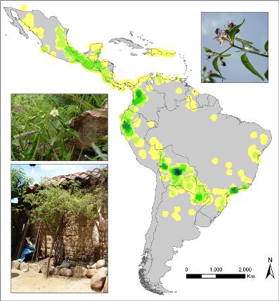
Observed richness of wild Capsicum species. |
Abstract
Ecogeographic studies provide critical information on plant genetic resources (PGR) to assess their current conservation status and prioritize areas for conservation. They have also proven useful for effective genebank management, such as the definition of core collections and identification of collection gaps. Geographic information systems (GIS) are useful tools for mapping ecogeographic distributions of biodiversity. GIS allow complex analyses to be performed, as well as clearly visualizing results in maps, which facilitates decision making and implementation of conservation policies by authorities.
Technological advances in both software and hardware, together with the increased availability and accessibility of geographical, environmental and biodiversity data through the internet, have led to increased application of GIS analyses for conservation and use of PGR in the last two decades. In this update, we give an overview of relevant techniques and advances in ecogeographic studies of PGR to analyse biodiversity data based on collected data and to target further collection. We commence with providing some general recommendations that are important when setting up new research projects that are aimed at assessing the conservation status of PGR and/or monitoring trends in (agricultural) biodiversity on the basis of ecogeographic data.
A brief introduction of commonly used methods and techniques for the analysis of inter- and intraspecific diversity is provided, including multivariate methods such as clustering and ordination. We also elaborate mapping of (agricultural) biodiversity data and emphasize the importance of ensuring good data quality. Furthermore, we provide a synopsis of available methods for distribution modelling and present an overview of useful open-access and commercial statistical and GIS packages. We conclude our update with an identification of future challenges and research needs.
Introduction
Ecogeographic studies refer to the process of collecting, characterizing, systemizing and analysing different kinds of data pertaining to target taxa within a defined region (Maxted et al. 1995). These kinds of studies are important for the formulation and implementation of more targeted and, hence, more effective conservation strategies for plant genetic resources (PGR) (Guarino et al. 2005). Taxonomic, morphological and genetic data can provide critical information about the diversity present in specific geographic areas, which, in turn, can be used for various purposes, such as the assessment of the current conservation status of PGR and to prioritize areas for in situ conservation. At the ex situ level, combining climate and other ecological information of an accession’s collection site – from its passport data – with corresponding morphological or molecular characterization data has also proven useful for effective genebank management (e.g., definition of core collections, identification of collection gaps, etc.). Geographic information systems (GIS) are useful tools for this type of analysis (Guarino et al. 2002). GIS tools allow complex analyses to be done, as well as visualizing results in clear maps, which facilitates decision making by relevant authorities and encourages the development and implementation of conservation policies (Jarvis et al. 2010). GIS analysis is carried out on the basis of coordinate systems; hence, the importance of georeferenced biodiversity data in ecogeographic studies.
The analytical approaches presented in chapters 15 and 16 of the 1995 edition of the Technical Guidelines are still valid. However, since 1995, technological advances and the growing availability of computers and portable global positioning system (GPS) receivers have led to the increased application of GIS analyses at various levels (including spatial data collected by rural communities and forest dwellers). The number and power of statistical programmes have also become much more advanced, especially with respect to analysis of genetic diversity (Holderegger et al. 2010). Furthermore, the general accessibility and use of the internet has created a leap forward in the sharing of geographical, environmental and biodiversity data. One of the notable examples is the Global Biodiversity Information Facility (GBIF) (www.gbif.org), a platform providing public access to biodiversity data from national museums, herbaria and genebanks worldwide. In October 2010, the GBIF contained roughly 39 million georeferenced plant observations.
Current status
Preliminary data handling
The following three paragraphs present several key recommendations on how to initiate an ecogeographic survey for PGR, following Guarino et al. (2005). Any such study should start with a commission statement that clearly states the objectives and the methodological design, including a sound strategy for data collection. Taxonomical experts should be identified who can provide key information about the target taxa and validate the results/products obtained from ecogeographic analyses and research, such as distribution maps and the results of collection gap analysis (Ramirez-Villegas et al. 2010). When available, it can be extremely useful to involve networks of taxonomical experts in such studies. Experts from the Latin American Forest Genetic Resources Network (LAFORGEN) have, for example, provided basic information about reproductive behaviour (breeding systems, pollination and seed dispersal systems) of prioritized tree species in the MAPFORGEN project (www.mapforgen.org).
Given the continuous changes in taxonomical classification of plants (APG III 2009), it is of utmost importance to determine upfront the taxonomical boundaries and nomenclature that will be used. The online database of the US Germplasm Resources Information Network (GRIN) (www.ars-grin.gov/cgi-bin/npgs/html/index.pl) provides a useful reference in this respect. All the same, it is strongly advisable to consult other databases such as the Plant List (www.theplantlist.org) or the International Plant Names Index (IPNI) (www.ipni.org) as well as to refer to other data sources such as experts, monographs and Floras.
The geographical extent and boundaries of the target region depend on the objectives of the study. For example, a study focused on assessing the status of PGR for strengthening national conservation programmes will be limited to the country’s national territory. In most other cases, since the occurrence of cultivated and wild taxa does not follow political boundaries, the target region of ecogeographic studies will be defined based on available knowledge about the distribution and diversity of taxa, compiled from literature reviews (e.g., Zeven and De Wet 1982) and consultation with experts from national or international agricultural research centres.
Data collection
Before starting actual collection of field data, preparation of a clear list of descriptors for passport data is recommended. In order for data from different studies and sources to be comparable, data collection, compilation and management require standardization. Data standards for multicrop descriptors have been developed to standardize passport data, morphological characterization and evaluation. These standards make the resulting information comparable across germplasm samples (Alercia et al. 2001). In a similar manner, in order to enable comparison of molecular characterization of crop species, minimum standard sets of markers have been suggested (Van Damme et al. 2010).
Original fieldnotes should be saved carefully and adequately backed up to allow for cross-checking of data at a later stage. A backup should also be made of the original data files stored in a notebook or GPS receiver. Field data can be integrated with additional data retrieved from online portals with data from genebanks and herbaria, contributing to more comprehensive analyses on the distribution and conservation of PGR (see table 15/16.1 for an overview).
Table 15/16.1: Online PGR Documentation Systems and Portals for Sharing Biodiversity Data
|
Portal |
Data type |
Website |
|
Germplasm Resources Information Network (GRIN), National Plant Germplasm System (NPGS) |
Passport, characterization and taxonomic information of PGR conserved by the United States Department of Agriculture (USDA) |
www.ars-grin.gov/npgs/index.html
|
|
System-wide Information Network for Genetic Resources (SINGER) |
Passport data of the PGR conserved by the Consultative Group on International Agricultural Research (CGIAR) Centres |
|
|
EURISCO |
Access to all ex situ PGR information in Europe. |
|
|
Genesys |
Passport, characterization and evaluation data for the 22 most important crops, from CGIAR Centres, EURISCO and GRIN |
|
|
Global Biodiversity Information Facility (GBIF) |
Passport data from herbaria and genebanks from all around the world |
|
|
SpeciesLink |
Passport data from the Brazilian herbarium information system |
|
|
JSTOR Plant Sciences |
Taxonomic information and historic herbarium samples |
|
|
Botanical Research and Herbarium Management System (BRAHMS) |
Instructions for mapping species distribution summaries and diversity indices |
Recording geographical data is normally done directly in the field by assigning geographical coordinates through the use of a GPS receiver. The geographic coordinate system in GPS receivers can usually be adjusted according to the user’s preferences. Two commonly used systems are longitude/latitude and Universal Transverse Mercator (UTM). Longitude/latitude is preferred in large-scale studies, such as for taxa that occur across different countries. The longitude/latitude coordinate system in combination with the World Geodetic System (WGS) 1984 is recommended in the data standards for multicrop descriptors (Alercia et al. 2001) and is the coordinate system of many freely available spatial datasets (see table 15/16.2 for an overview), which makes it the preferred option in combination with WGS 1984 for easily combining different spatial datasets. For studies at lower administrative units (e.g., province, department, state), the UTM may be preferred because of the low distortion at this scale and the ease in calculating geographic distances. To be able to carry out GIS analysis with the collected data, longitude/latitude coordinates should be in decimal degrees. If longitude/latitude coordinates of collection sites have been listed in degrees, minutes and seconds, a special formula can be applied to convert these coordinates into decimal degrees (see chapter 2 of Scheldeman and van Zonneveld 2010) .
Table 15/16.2: Some Spatial Data Sources and Tools
|
Climate |
|
|
Topography |
|
|
Remote sensing (satellite) |
|
|
Soils |
|
|
Other spatial data |
|
Since various identification codes may be used in the different steps of collecting, characterizing and evaluating germplasm material (e.g., collector code, field code, collection code), it is essential to clearly define a unique identification code to be applied to each accession throughout the entire study. This will ensure consistent and unequivocal correspondence between each accession and the complexity of its passport, characterization and evaluation data. It is key to getting confident georeferenced taxonomic, phenotypic or genetic diversity data for ecogeographic studies. The addition of new codes should be considered carefully because more codes may lead to confusion and increase the likelihood of making errors in the documentation system, thus affecting the reliability of the data and reducing the possibility of effectively conserving and using collected and characterized germplasm.
Diversity analyses
Ecogeographic studies related to the conservation and use of PGR are mostly focused at the species or gene level of plant diversity. At the species level, the observed unit of alpha diversity is the species, measured mostly as present or absent in a certain location (species richness). Other parameters of species diversity are evenness and abundance (Magurran 1988). Studies at the gene level can be either interspecific (e.g., phylogenetic studies within a gene pool or clade) and/or intraspecific (i.e., to understand genetic variation between plant individuals of the same species or within and between populations of plant species). For the purpose of measuring genetic variation, the chosen units of diversity may be phenotypic traits (the products of a gene or its expression) or, more directly, variation in sequences of neutral or functional portions of DNA or RNA, measured with the assistance of molecular markers (e.g., SSRs, SNPs, DArT, AFLPs; see De Vicente and Fulton [2004] for an overview of different types of molecular markers).
Richness in species or in the number of alternating DNA sequences in specific parts of a plant species genome (e.g., allelic richness) are straightforward measures of diversity and are commonly used for prioritizing conservation areas of either plant communities – based on number and uniqueness of observed species (Gotelli and Colwell 2001) – or within-species populations identified through molecular markers (Frankel et al. 1995a; Petit et al. 1998). However, richness is sensitive to sample bias – the situation where an uneven number of observations or collections has been made across the sampling units included in an ecogeographic study (some units will contain more observations than others). The rarefaction methodology allows correcting such sample bias by recalculating richness on the basis of an equal, user-defined number of observations per sampling unit (Gotelli and Colwell 2001; Petit et al. 1998).
In studies of genetic diversity based on molecular markers, the number of locally common alleles is an important indicator for prioritizing populations of wild and domesticated plant species for in situ conservation. These alleles occur in relatively high frequency over a limited area and can indicate local adaptation to specific environments (Frankel et al. 1995a). Locally common alleles can be identified by statistical programmes for genetic data such as GenAlEx (see table 15/16.3), which identifies alleles with a frequency higher than 5% in a local population and occurring in less than 25% of all populations as locally common alleles (Peakall and Smouse 2006). Another way to detect locally common alleles is with the help of GIS, by identifying those alleles that occur at relatively high frequencies within a given maximum distance (see chapter 5 of Scheldeman and van Zonneveld 2010).
Distance parameters
In diversity analysis, ecological and genetic distances are statistics of central importance that allow investigating the existence of structure and patterns in biodiversity data (beta diversity). This, in turn, is essential for prioritization strategies for in situ conservation (Gallo et al. 2009; Petit et al. 1998; van Zonneveld et al. in prep.), as well as for germplasm management and use, such as in the establishment of core and reserve collections (Frankel et al. 1995b). Ecological distances can be used to calculate how divergent different sampling units are, based on their species or varietal composition, whereas genetic distances are typically used to calculate how divergent within-species individuals or populations are, based on morphological trait or allelic composition. Genetic distances can also be used in phylogenetic studies to order species. Multivariate techniques such as clustering and ordination allow the ordering of units of diversity, such as sampling units, species, plant individuals (within species), on the basis of the ecological or genetic distances between them. Several open-access analysis packages can be useful for carrying out diversity analysis, including the calculation of distance parameters, clustering and/or ordination analyses. Some commonly used programmes for ecological and genetic diversity and structure analysis are listed in table 15/16.3. Additional software for specific genetic analyses is listed in Appendix A of Lowe et al. (2004) and in Excoffier and Heckel (2006).
There is a wide variety of different distance statistics that can be employed, each with different properties. Some distance measures, such as Euclidean distance, are used for calculating both ecological and genetic distances, whereas other measures are generally used for either one of them. Other popular ecological distances include Bray-Curtis, Kulczynski, Hellinger and Chi-square distances (Kindt and Coe 2005). Since the distance measure is the input for subsequent multivariate techniques (e.g., clustering, ordination) and will thus affect the results of this type of analyses, it is important to select an appropriate distance statistic from the start. A desirable characteristic of any ecological distance parameter is that it assigns the same maximum distance to all pairs of sites that do not share any species (e.g., a property of the Bray-Curtis and Kulczynski distances [Kindt and Coe 2005]). For other features of different ecological distance parameters and how to test them, refer to Kindt and Coe (2005).
Table 15/16.3: Open-Access Applications for Biodiversity and Genetic Analysis
|
Software |
Properties and applications |
Source |
|
Biodiversity. R |
A single software environment for performing nearly all types of biodiversity analysis; Operates in statistical programme R |
Kindt and Coe 2005
|
|
Vegan |
Ordination methods, diversity analysis and other functions for community and vegetation ecologists; Operates in statistical programme R |
Kindt and Coe 2005 http://cran.r-project.org/web/packages/vegan/vignettes/intro-vegan.pdf |
|
Biodiversity-Pro |
Alpha and beta diversity analysis, multivariate statistics |
McAleece et al. 1997 http://gcmd.nasa.gov/records/NHML_Biopro.html |
|
EcoSim |
Null model analysis in community ecology |
Gotelli and Entsminger 2004 http://garyentsminger.com/ecosim/index.htm |
|
PAST |
Developed for paleontology, but offering vast possibilities for (multivariate) biodiversity analysis |
Hammer et al. 2001 http://folk.uio.no/ohammer/past |
|
GenStat Discovery |
Free version of statistical programme GenStat |
|
|
Adegenet |
Population genetics, including clustering based on Bayesian Information criterion, Discriminant Analysis of Principal Components and spatial Principal Components Analysis; Operates in statistical programme R |
Jombart 2008 http://adegenet.r-forge.r-project.org |
|
Structure |
Free software package for using multi-locus genotype data to investigate population structure. |
Pritchard et al. 2000 http://pritch.bsd.uchicago.edu/structure.html |
|
GenAlEx |
User-friendly cross-platform package for population genetic analysis Runs within Excel |
Peakall and Smouse 2006 www.anu.edu.au/BoZo/GenAlEx |
The choice of genetic distance measures largely depends on the type of data (phenotypic, or dominant or co-dominant molecular marker data) and whether distance is calculated between individuals or between groups of individuals. A guide to which measures of genetic distances may be most appropriate for different situations is provided by Lowe et al. (2004) and De Vicente et al. (2004b). Popular genetic distance parameters include Nei’s standard genetic distance, the Arc distance or the Manhattan distance for quantifying distances between populations, and the Tanimoto or Jaccard distance for quantifying distances between individuals (Geburek and Turok 2005).
A series of distance parameters can be used when estimating the variation in phenotypic traits between individuals of the same species. This applies to data analyses from so-called “common garden” experiments (e.g., Willemen et al. 2007). In such experiments, plant material collected in different sites is established in field trials under a common environment, in order to reduce the variance by the environmental effect in the expression of phenotypic traits. When a dataset contains both nominal and continuous morphological data, the Gower distance can be used (Grum and Atieno 2007; Willemen et al. 2007). The Ward-MLM distance (Franco et al. 2010) is useful for combining phenotypic and molecular marker data in clustering or ordination. In light of the different properties of the different genetic distance statistics, it is important to note that care must be taken when comparing different studies that use different distance parameters (Finkeldey 2005).
Distance measures can also be used to test the hypothesis that individuals located further away from each other are also genetically more distant. To do this, Mantel correlation is often used to calculate between pair-wise geographical and genetic distances. Mantel tests can be carried out in packages like Adegenet or GenAlEx (see table 15/16.3). Other types of distances can be compared with genetic distances through Mantel tests as well, such as environmental distances, like climate or soil, to examine whether individuals from different ecological zones are also genetically more distinct (Kozak et al. 2008). In GIS programmes, environmental data (climate, topography, soils) for each collection site can be easily extracted from freely available spatial data maps and exported to a spreadsheet for further statistical analysis (Scheldeman and van Zonneveld 2010). Table 15/16.2 provides an overview of important sources and tools for spatial data.
Clustering
Clustering refers to methods that draw on the distance parameters discussed above for assigning units of diversity such as sampling units, species, within-species individuals or populations, into groups or clusters whose members show a certain level of similarity for measured characteristics. Many hierarchical and non-hierarchical clustering methods exist and it is practically impossible to choose a “best” method because of their heuristic nature. The value of clustering is limited because the outcomes can change substantially depending on different combinations of distance parameters and clustering methods. Therefore, this type of analysis is useful for exploring variation within collected data, but it should not be considered as definitive proof of clear patterns in data (Kindt and Coe 2005). Whereas a markedly discontinuous structure in data will likely be detected by almost any method, a more gradual or continuous structure will be more difficult to detect by cluster analyses (Jongman et al. 1995) and ordination methods are in these cases more appropriate than clustering methods (Kindt and Coe 2005). It is possible to evaluate the clustering performance of a distance statistic by calculating the cophenetic correlation, which compares the distances between observation points calculated by a given distance parameter with the corresponding distances between these points in the cluster diagram (for further information see Kindt and Coe [2005]).
Grum and Atieno (2007) provide a user-friendly introduction to clustering with continuous and nominal variables in the free statistical programme R. A frequently used programme to assign plant individuals to genetic clusters on the basis of molecular markers is Structure (Pritchard et al. 2000), which uses a Bayesian approach to determine the probabilities of plant individuals belonging to each cluster from a predefined number of clusters. Evanno et al. (2005) present a method to determine, within the Structure environment, the number of clusters that best describe the genetic structure of the gene pool. These clusters can also be geographically visualized in GIS (Vigouroux et al. 2008).
Ordination
The basic aim of ordination is to represent observations (e.g., different species across a climate gradient, or allelic composition of within-species plant individuals) and sampling units (e.g., different plots in which species composition is determined, or sample tissues from different individuals that are used for determining allelic composition) in a two-dimensional space in such a way that points that are close together are more similar than points that are further apart. Ordination allows simultaneous representation of observations and sampling units on the same plane. Observations of species or plant individuals (within a species) that are plotted close together have a higher likelihood to occur in sampling units with more similar characteristics (e.g., because they share the same environmental niche or morphological or molecular characteristics) as compared to points that are plotted further apart. Likewise, points representing sampling units that are close together correspond to sampling units that are similar in species, morphological trait or allelic composition, whereas points that are far apart correspond to samples that are dissimilar in this respect. This combined visualization allows one to relate patterns in observations with underlying patterns in the relative sampling units (for instance, between-species similarity and similarity between the plots where these species were observed).
Two general approaches are used in ordination. In direct (or constrained) gradient analysis, direct relationships are sought between (1) the occurrence and/or abundance of species, varieties or alleles and (2) specifically measured (environmental) variables that characterize the sampling units in which these species, varieties or alleles were observed. Observations and sampling units are arranged in a virtual space along axes that are linear combinations of these explanatory variables (e.g., environmental variables), and the predictive power of each of the respective variables is determined (Höft et al. 1999). By contrast, indirect (or unconstrained) gradient analysis focuses entirely on observations and allows maximum explanation of variation without the restriction of explanatory variables (Jongman et al. 1995). This type of analysis is particularly useful when there is no clear foreknowledge about variables that might explain variation between the observations.
Most types of direct and indirect gradient analysis can be divided into two main types of ordination techniques: those that are related to (1) a linear (monotonic) response model in which the abundance of any observational unit (such as species or within-species plant individuals) either increases or decreases with the value of each of the explanatory variables (e.g., Principal Components Analysis [PCA] and Redundancy Analysis [RDA]) and (2) a unimodal response model, where any observational unit occurs within a limited range of the explanatory variables (e.g., Correspondence Analysis [CA] and Canonical Correspondence Analysis [CCA]) (Jongman et al. 1995). Given that the unimodal distribution is more common in nature than a linear distribution, it might be more advantageous to use unimodal over linear response models (Kindt and Coe 2005). According to Jongman et al. (1995), it is advisable to start analyzing biodiversity data by using unimodal models (CA, Detrended Correspondence Analysis [DCA] or CCA) and to decide afterwards whether one could simplify the model to a monotonic one. Non-metric multidimensional scaling (NMDS) is an additional method for indirect gradient analysis that differs in various ways from nearly all other ordination techniques. It can handle non-linear species responses of any shape and allows the use of any distance parameter (Holland 2008). Table 15/16.4 provides a summary of the different options of ordination techniques.
Table 15/16.4: Ordination Techniques
|
Unconstrained or indirect gradient analysis |
Constrained or direct gradient analysis |
Distance measure |
|
|
Unimodal response model |
|
|
Chi-square distance |
|
|
Chi-square distance |
|
|
Monotonic or linear response model |
|
|
Euclidean distance |
|
|
Any distance |
|
|
Non-linear response of any shape |
|
Any distance |
Mapping ecogeographic data
Data quality control
In mapping the ecogeographic distribution of the target taxa, it is crucial for the data to be of high quality and precise (i.e., to contain a minimum number of errors at a specified scale of study). Therefore it is very important to check the quality of the data before they are used in analysis. During field collection, it is recommended that detailed passport information be noted down in a field book and that this original information be carefully saved to enable any error that might emerge during data analyses to be tracked back. Chapman (2005a,b) and chapter 4 of Scheldeman and van Zonneveld (2010) explain several ways to check the quality of georeferenced data, including verification of consistency between the data on (1) the administrative unit (country, provinces, departments) mentioned in the passport data of a collection or observational record as it was registered in the field and (2) the administrative unit in which it is mapped in a GIS programme.
Another way to identify potentially erroneous points is to carry out an outlier analysis, which identifies georeferenced records of the target taxa that are located in atypical climates compared to the climatic niche in which records of the taxa normally occur (Scheldeman and van Zonneveld 2010). Such records can be erroneous due to incorrect coordinates or taxonomic misidentification. However, they might also effectively represent individuals at the marginal ends of a taxon’s distribution range, which could contain valuable traits for adaptation to atypical site conditions. Yet another possibility is that areas with a distinct climate, where outliers are located, have been undersampled in comparison to other areas. If this is the case, these areas could be considered for further collection. For these reasons, when possible, it is recommended that the field book containing original passport information of a record in an atypical climate be consulted (or contact the collector in case the data came from a third party) to find out whether the record is an error. If the outlier appears not to be an error, it can be useful to further evaluate the properties of the plant individuals located in the outlier location based on molecular or phenotypic characterization. If plant individuals possess properties of human interest, it can be worth considering further exploration of the surrounding areas for other plant individuals/populations with similarly interesting traits.
One should also bear in mind that in many cases, data originating from herbaria and genebanks (e.g., freely available from GBIF) were not generated for the purpose of biogeographic studies, and they are often the result of ad hoc collecting or non-systematic and uneven sampling efforts (Chapman 2005a). Frequently, specimens/accessions have been collected mostly or exclusively from areas that are easily accessible or where a taxon is known to occur, thus negatively affecting the representativeness of the data (Hijmans et al. 2000). Such sample bias can later be corrected – although only to a certain extent – with methods such as rarefaction and distribution modelling (see Scheldeman and van Zonneveld [2010] for further details). The best way to prevent sample bias is, of course, by establishing a sound strategy for data collection, although it should be acknowledged that this is not always possible.
Georeferencing
Georeferencing, which assigns geographical coordinates to collection records or observation data missing such coordinates, can substantially increase the number of sound observation records of the target taxa and consequently improve the quality of ecogeographic studies. Specimen label data from collections such as herbaria, which do not include geographical coordinates but do include precise information about the locality where the specimen was collected or observed, can be georeferenced using either gazetteers that can be downloaded from the DIVA-GIS website (see table 15/16.2) or automated online gazetteers such as GeoNames (www.geonames.org) and BioGeomancer (www.biogeomancer.org). Google Earth can be useful for georeferencing records as well, especially those that are taken at a specific distance along the road between two localities. BioGeomancer provides a significant step towards automated georeferencing: it currently encompasses natural language processing (geo-parsing) to interpret the descriptive locality text, place-name lookup to register localities with known geographic coordinates, and ambiguity analysis to self-document uncertainties in resulting geographic descriptions. At the time of this publication, work was still in progress for a workbench that will allow georeferencing of batches of data, speeding up the handling of large bodies of observation records.
Plant diversity, distribution and conservation
The number and frequency of species, varieties or alleles in distinct sampling units within a study area (alpha diversity) are the principal subjects of the spatial analysis of diversity to prioritize areas for conservation in situ and collection of PGR. Sampling units may refer to previously identified sites, administrative units or grid cells of any chosen size. In many cases, such as the example in chapter 15 of the 1995 edition of the Technical Guidelines, species distribution is mapped on the basis of observed species presence in the cells of a grid that covers the study area. At a national or continental level, this grid size may be as large as 50 x 50 km, as used in the Atlas Florae Europaeae (2011), or 100 x 100 km (about one degree) (Scheldeman et al. 2007). In this respect chapter 5 of Scheldeman and van Zonneveld (2010) provides working examples to practice mapping species and allelic richness in grid cells with a point to grid analysis in DIVA-GIS.
The advantage of using grid cells is that these allow the comparison of diversity between sampling units of similar geographical size throughout the extent of the study area. DIVA-GIS and other GIS programmes –among those reviewed in Steiniger and Bocher (2008) – can be used to carry out grid-based diversity analysis (see table 15/16.5 for open-access and commercial packages) and have been applied in several studies to assess the distribution and conservation status of crop gene pools (e.g., Hijmans and Spooner 2001; Jarvis et al. 2003; Scheldeman et al. 2007). Other ways to map distribution and richness are by means of circular area (Hijmans and Spooner 2001) or circular neighbourhood (Hijmans et al. 2005b; Scheldeman and van Zonneveld 2010).
Methods have been developed to optimize the number of conservation areas based on the number of species, varieties or alleles in different units and how they complement each other. DIVA-GIS also includes a reserve selection algorithm, developed by Rebelo and Siegfried (1992), which calculates the minimum number of areas (grid cells) necessary to conserve a given number of species, varieties or alleles of the gene pool under study (Hijmans et al. 2001). It ranks grid cells that should be given priority for conservation in the following order: first priority is given to the grid cell with the highest alpha diversity; subsequent priority is given to those grid cells that best complement the initial ones because they contain the highest number of new species, varieties or alleles that were not found in the previously selected grid cells (beta diversity). Chapter five of Scheldeman and van Zonneveld (2010) explains how to carry out such a reserve selection.
Distribution modelling
For most plant species, including many crop wild relatives and socioeconomically important tree species, only a limited amount of information on their natural distribution is currently available (Nic Lughadha et al. 2005). Distribution modelling or ecological niche modelling is considered a useful tool for overcoming the lack of concrete information on the natural distribution of species (Guarino et al. 2002; Hernandez et al. 2006). It aims to distinguish between zones where the species could potentially occur (i.e., areas with similar environmental conditions to the defined ecological niche) and areas where the species is likely to be absent because the local environment is different from the ecological niche. Distribution models can thus be used to predict the full natural distribution ranges for plant species on the basis of records of presence and absence by defining the ecological niche of a species on the basis of statistical (empirical) relations between occurrence and environmental factors. GIS are very useful in this respect because they allow extraction of information from environmental data layers relative to sites where a species has been observed, as well as to sites where it is known to be absent, and allows visualizing and editing the outcomes of the model on a map. Environmental data layers in distribution modelling can be derived from datasets like those listed in table 15/16.2. Depending on the modelling programme used, they can consist of only continuous variables, such as climate data derived from WorldClim (Hijmans et al. 2005a), or also include nominal variables, such as maps of vegetation or soil type. While distribution modelling is traditionally used to predict the distribution of species, it can also be applied for intraspecific units of diversity, such as ecotypes or clusters defined on the basis of morphological or molecular markers.
The collection of absence records is a challenge because the reasons for absence are not always clear; it might either be due to ecological characteristics, human disturbance or simply because species presence was overlooked during an inventory or collection. Therefore, distribution modelling often uses presence records only (Pearce and Boyce 2006). Presence records can be derived from herbarium specimens, genebank accessions or vegetation/plant species inventories, which have become increasingly available online through portals such as GBIF (see table 15/16.1).
In addition to understanding the full distribution range of a species, distribution models have also been used in gap analyses to prioritize areas for germplasm collection (Jarvis et al. 2005; Scheldeman et al. 2007). In this respect, a gap refers to a location where a distribution model predicts the potential occurrence of a target taxon, but where specimens and/or germplasm of the taxon have not actually been collected. Ramirez-Villegas et al. (2010) present a method based on the identification of sampling, geographic and environmental gaps to prioritize among taxa. Chapter 6 of Scheldeman and van Zonneveld (2010) explains how to carry out a gap analysis with the use of the distribution modelling programmes Maxent and DIVA-GIS. An important source of guidance is the GapAnalysis portal (http://gisweb.ciat.cgiar.org/GapAnalysis) with its methods for crops and crop wild relatives.
Table 15/16.5: GIS Packages
|
Open-source desktop GIS |
Properties |
Source |
|
DIVA-GIS |
Biodiversity analysis, species distribution mapping, etc. Also provides free spatial data for the whole world |
|
|
GRASS (Geographic Resources Analysis Support System) |
Analysis and scientific visualization, cartography, simulation |
|
|
QGIS (Quantum GIS) |
Viewing, GRASS-Graphical User Interface |
|
|
uDig (User-friendly Desktop Internet GIS) |
Viewing, editing, analysis |
|
|
SAGA (System for Automated Geoscientific Analyses) |
Analysis, modelling, scientific visualization |
|
|
ILWIS (Integrated Land and Water Information System) |
Analysis, integrating image, vector and thematic data |
www.itc.nl/Pub/Home/Research/Research_output/ILWIS_-_Remote_Sensing_and_GIS_software.html |
|
OpenJUMP 2002/03 |
Editing, analysis JUMP Family (Java Unified Mapping Platform) |
|
|
Commercial GIS |
Properties |
Source |
|
Esri |
Products include ArcView 3.x, ArcGIS, ArcSDE, ArcIMS, ArcWeb services and ArcGIS Server. |
www.esri.com |
|
Autodesk |
Products include Map 3D, Topobase, MapGuide and other products that interface with its flagship AutoCAD software package |
http://students.autodesk.com/?nd=download_center&c_key=31305F5F416D657269636173& |
|
Bentley Systems |
Include Bentley Map, Bentley Map View and other products that interface with its flagship MicroStation software package |
|
|
ERDAS IMAGINE |
Products by ERDAS Inc, include ERDAS ER Mapper, ERDAS ECW JPEG2000 SDK |
www.erdas.com/products/ERDASIMAGINE/ERDASIMAGINE/Details.aspx |
|
Intergraph |
Products include G/Technology, GeoMedia, GeoMedia Professional, GeoMedia WebMap, and add-on products for industry sectors, as well as photogrammetry |
|
|
MapInfo |
Products by Pitney Bowes, include MapInfo Professional and MapXtreme |
|
|
Smallworld and Spatial Eye |
Purchased by General Electric and used primarily by public utilities |
http://site.ge-energy.com/prod_serv/products/gis_software_2010/en/index.htm |
Another application of distribution modelling is to examine the impact of climate change on the distribution of plant species of interest and socioeconomic importance, such as crop wild relatives (Jarvis et al. 2008) or timber tree species (Saénz-Romero et al. 2006;van Zonneveld et al. 2009a).
It is important to note that distribution modelling can be used to better understand species distribution and to help prioritize areas for germplasm collection only when some information about a species is already available. There is no standard in terms of the minimum number of observation points required, as this will often relate to the nature of the species: for rare species or species with a restricted niche, only a small number of presence records may be sufficient, while for species with a broad niche and extensive distribution range, a higher total number of records is desirable. Although it is difficult to provide strict guidelines on the minimum number of presence records necessary for credible distribution modelling, a number of illustrative examples exist:
-
Scheldeman et al. (2007) used a minimum of 10 points for rare Vasconcellea species with a known restricted distribution.
-
The MAPFORGEN project (MAPFORGEN 2011), which evaluates the natural distribution of 100 species native to Latin America, used a minimum number of 20 species presence records.
-
van Zonneveld et al. (2009b) worked with a minimum number of 50 presence records for two pine species with a broad geographic distribution range throughout Southeast Asia.
Modelling a species’ natural distribution is done under several conditions, the most important being (1) the species should be in a state of equilibrium with its environment (in other words, the environmental ranges are restricted by competition and predation and not by dispersion limitations) and (2) the available environmental variables (e.g., climate variables) used in the modelling are determinant a-biotic factors in shaping the natural distribution of the species. In practice, one or both of these conditions are often not met; nonetheless, distribution modelling is still a useful tool for approximating the natural distribution of a species and, as such, is relevant for prioritizing conservation activities.
Because the model outcomes are an approximation of the species’ real distribution, it remains a challenge to estimate how representative modelled distributions are. Moreover, the outcomes of distribution modelling can vary depending on the modelling program used, quality of presence records and included environmental layers. The outcomes of these models, although potentially useful, should therefore be validated carefully for in situ conservation planning and targeted collection (Loiselle et al. 2003). There is extensive literature about methods for validating models (e.g., Araújo et al. 2005; Beauvais et al. 2006). DIVA-GIS includes an option to calculate two frequently used indicators of model evaluation – maximum Kappa and Area Under Curve (AUC) of Receiver Operation Curve (ROC) – from cross-validating modelled distribution maps with a subset of the presence records (Hijmans et al. 2005b). Maxent also provides an option to calculate AUC (Phillips 2009), albeit it is argued that other indicators are more appropriate to measure model performance (see Lobo et al. 2008).
Over the years, a wide variety of ecological distribution models have been described in the literature, an exhaustive description of which is beyond the scope of this chapter. In the following section, we give a brief overview of the most popular empirical distribution models that are based on observed data and which assume an equilibrium state of the ecosystem, partly based on Peters (2008).
-
Linear Regression models: Regression analysis aims at predicting the pattern in one response variable from the pattern of one or several independent or predictor variables (Kindt and Coe 2005).
-
General linear models (GLMs): General linear models were developed for situations when certain aspects of the linear regression model are not appropriate. GLMs provide ways of realistically estimating a function of the mean response (the so-called link function) as a linear combination of a given set of predictor variables (Dobson 2002; Nelder and Wedderburn 1972). Popular GLM models are the Poisson GLM with a logarithmic link function (when data are counts) and the binomial GLM with logit link function (for presence-absence data) (Kindt and Coe 2005).
-
General additive model (GAM): The general additive model extends the GLM by fitting nonparametric smoothing functions to estimate relationships between the response and the predictive variables (Hastie and Tibshirani 1986). The smoothing function generates a curve that can flow more freely between the data than a straight line.
-
Tree-based techniques: Tree-based techniques partition the predictor (environmental) space into parts and then fit a simple model to each part. Classification (categorical response) and regression (continuous response) trees (CART) (Breiman et al. 1984) are a popular technique. Other methods, such as rule-based classification (Lenihan and Neilson 1993) and maximum likelihood classification (Franklin and Wilson 1991), have been developed. Random Forests is a related technique that differs from ordinary tree-based techniques in that it generates an ensemble of trees instead of a single best tree (Breiman 2001).
-
Bayesian techniques: Distribution models based on Bayes’ theorem modify an initial (a priori) estimate of the probability of encountering a species or vegetation type in the landscape by using (1) known preferences (e.g., based on expert knowledge or the literature) of the species or vegetation type for environmental characteristics and (2) information concerning the distribution of these characteristics in the landscape (Guisan and Zimmerman 2000; Tucker et al 1997). However, the quality of the a priori information largely determines the model’s performance.
As mentioned above, this list of techniques is not exhaustive; many others exist, including artificial neural networks (Lek and Guegan 1999), support vector machines (Cortes and Vapnik 1995), the environmental envelope (Busby 1991) and maximum entropy (Elith et al. 2011; Phillips et al. 2006) models.
In terms of software packages, Maxent, which implements a maximum entropy modelling approach, has performed very well in comparison to others (Elith et al. 2006; Hernandez et al. 2006). It has been used to evaluate the outcomes of species distribution models under different sets of environmental layers (Blach-Overgaard et al. 2010) and to compare the outcomes of species distribution model with the use of different presence record datasets (Feely and Silman 2011). Integrated into DIVA-GIS are other two distribution modelling programmes: BIOCLIM and DOMAIN (Carpenter et al. 1993; Hijmans et al. 2005b). Although their statistical algorithms are easier to understand than the one used by Maxent, they have not performed as well in comparative studies (Elith et al. 2006; Hernandez et al. 2006). An advantage of Maxent and Domain is that they allow the inclusion of both continuous variables, such as climate data, and categorical variables, such as layers of vegetation and soil types; BIOCLIM only allows the inclusion of continuous variables. Table 15/16.6 lists some software packages that are commonly used for distribution modelling.
Table 15/16.6: Distribution Modelling Packages
|
Software |
Properties and applications |
Source |
|
Maxent |
Maximum-entropy approach for distribution modelling |
|
|
BIOMOD |
Ensemble forecasting of species distributions, enabling the treatment of a range of methodological uncertainties and the examination of species-environment relationships |
|
|
OpenModeller |
Cross-platform environment where a fundamental niche modelling experiment can be carried out A number of algorithms are provided as plug-ins, including GARP, Climate Space Model, Bioclimatic Envelopes, Support Vector Machines and others |
|
|
Biomapper |
A kit of GIS and statistical tools designed to build distribution models and maps for any kind of animal or plant Centred on the Ecological Niche Factor Analysis (ENFA), which does not require absence data |
|
|
DOMAIN |
Can operate effectively using only records and a limited number of biophysical attributes |
Carpenter et al. 1993 |
|
Random Forests |
(See text above) |
|
|
GARP |
The Genetic Algorithm for Rule-set Prediction (GARP) is a distribution modelling method |
Stockwell and Peters 1999 |
Genetic structure and genecological zonation
Spatial patterns of genetic structure are traditionally visualized on spatial data maps by means of vector point data in different colours (e.g., Motamayor et al. 2008) and in pie charts (Trognitz et al. 2011). Pie charts are also used to display similarities and differences in the composition of chloroplast or mitochondrial DNA of different populations (Pautasso 2009). More recently, grid-based analyses based on molecular marker data have been used to develop accurate conservation strategies for PGR (Kiambi et al. 2008; van Zonneveld et al. in prep.) and to understand the origin and domestication of crops (van Etten and Hijmans 2010).
For most tree species and crop wild relatives, information concerning patterns of intra-specific diversity across their distributions, which can help in prioritizing areas for in situ conservation and germplasm collection, is not yet available. In such cases, genecological zonation can provide guidance with respect to the establishment of networks of conservation stands (Graudal et al. 1995). Following the assumption that ecogeographic variation shapes genetic patterns (Byers 2005; Ramanatha Rao and Hodgkin 2002), information about climatic and ecological parameters and topographic barriers can be used to define genecological zones, which putatively correspond to differences between species populations that are likely to be genetically distinct because of limited gene flow and/or local adaptation to specific environmental conditions. To identify different climate zones, for instance, DIVA-GIS can be used to map climate zones on the basis of the WorldClim dataset with the use of the clustering option (Hijmans et al. 2005b). Topographic barriers can be visualized with GIS and used to assign records to different populations separated by mountain ranges or water division lines (see table 15/16.2). Such theoretically constructed zones should ideally be validated by empirical data (ground-truth) in order to allow adjustment or refinement. When genetic (molecular or phenotypic) data exist, clustering or ordination techniques can be used to evaluate how much of the genetic structure can be explained by grouping plant individuals in populations according to genecological zones (e.g., Zhang et al. 2006).
Ecogeographic distribution data of specific taxa can provide measures of their plasticity and adaptation and can be a useful complement to morphological and molecular marker studies (or even serve as proxy if morphological or molecular data are not available). In this context, ecogeographic studies support the prioritization of material to be secured in genebanks (Parra-Quijano et al. 2011) and the establishment of core collections for breeding purposes. A programme like Powercore allows the inclusion of ecogeographic variables, such as climate (continuous) and watersheds (nominal), to calculate a subset that is assumed to be representative for a specific taxon in the complete collection (Kim et al. 2007). Ecogeographic studies are also used for carrying out gap analyses, and the higher the level of spatial coverage, the greater the amount of genetic variation that is likely to be captured. In recent years, methodologies and approaches for assessing gaps in genebank collections and prioritizing taxa to be searched in collection missions have been developed. Maxted et al. (2008) provide a gap analysis based on a combination of taxonomic, genetic and ecogeographic diversity.
When specific accessions from a genebank collection have shown interesting traits in evaluation trials (such as drought tolerance or pest and disease resistance), it can be worthwhile to evaluate genebank accessions collected in the same ecological zone since they will most likely have adapted to a similar environment and might express similar interesting traits. This approach, called Focused Identification of Germplasm Strategy (FIGS) has been used, for example, to pre-select 1320 accessions from a wheat collection of about 16,000, to screen on resistance to powdery mildew. Sixteen percent of the selected accessions showed resistance to the disease (Bhullar et al. 2009).
Monitoring trends in biodiversity
Information about species distribution can be used as an indicator to assess the conservation status of the natural populations of particular plant species. It can be anticipated that species with a narrow and/or fragmented natural distribution are more vulnerable to threats such as changes in land use and climate than species with an extensive and continuous distribution. The World Conservation Union (IUCN) has developed several Red List parameters that are based on species distribution, most notably, the extent of occurrence and area of occupancy (IUCN B criterion). In combination with criteria about observed or expected trends in population size, these parameters provide information about the conservation status of species (IUCN 2008). The distribution-based Red List parameters can be calculated with freely available GIS tools (Willis et al. 2003). In combination with information from species experts, they can be used to evaluate the conservation status of wild species, including crop wild relatives (e.g., VMABCC and Bioversity International 2009).
It is generally accepted that the modernization of agriculture and changes in land use could have a negative effect on the diversity of crop species and their wild relatives (agricultural biodiversity) conserved on farms and at a landscape level, and might lead to genetic erosion at the level of either crop, variety or allele (van de Wouw et al. 2010). Nevertheless, exact, well-quantified measures and evidence of genetic erosion as a consequence of agricultural modernization are scarce. Indeed, under certain conditions, crop diversity might even increase when modern varieties are introduced (Bioversity International 2009). Therefore, it is important to establish adequate indicators and to identify areas where agricultural biodiversity can be monitored. Genetic erosion of crops in specific study areas can be measured by comparing current in situ diversity with the diversity of genebank material collected from the same area in the past (De Haan et al. 2009). The existing genetic diversity can be compared between different types of land use, such as commercial agriculture vs. traditional farming to understand the dynamics in the use of crop diversity (van Heerwaarden et al. 2009). GIS are a useful tool to overlay areas of high crop diversity with thematic maps that provide information about accessibility, ethnicity and land use, among other variables, and to better understand which social and economic variables drive the dynamics in the use of crop diversity (e.g., Willemen et al. 2007)
In terms of indicators, those developed within the IUCN criteria may not be appropriate for monitoring the dynamics in the use of crop diversity since they are limited to monitoring at the species level (rather than intra-specific level). An indicator proposed by the Conference of the Parties to the Convention on Biological Diversity (www.cbd.int) is the total number and share of main crop varieties, but this might not adequately reflect relative changes in crop diversity (Eaton et al. 2006). From a scientific point of view, allelic evenness and richness measured through molecular markers are more appropriate for detecting changes in crop diversity (Eaton et al. 2006). Although molecular marker studies have become increasingly common and can be applied to monitoring trends in agricultural biodiversity, other, non-molecular-based indicators are also recommended (OECD 2003). These include the share of land devoted to non-intensive production/high biodiversity (with varieties specific to such production systems), percentage of seed of three major crops/varieties originating on-farm and number of traditional (low-production) varieties stored in a genebank (Eaton et al. 2006). The monitoring of crop diversity on the basis of commercial and traditional varieties might be particularly relevant for specific crops when a sound inventory of registered varieties is in place (Eaton et al. 2006) or when taxonomic keys to distinguish between crop varieties are defined and accepted, such as in the global project of native maize (Proyecto global de maíces nativos, www.biodiversidad.gob.mx/genes/proyectoMaices.html). However, registration of varieties according to morphological characterization may still lead to a substantial degree of misidentification (van de Wouw et al. 2011; Vigouroux et al. 2008). Since the results for molecular markers are more consistent, standardized sets of these markers (Van Damme et al. 2010) are recommended as indicators in monitoring crop diversity (van de Wouw et al. 2010). For molecular marker studies, young shoots or other vegetative material from individual plants can be collected in the field and simply stored in bags (such as Ziploc® bags) with silica gel before they are sent to a laboratory for molecular analysis.
The disadvantage of molecular markers is that in many cases, neutral diversity is measured within a sampling unit and not, directly, the diversity of genetic resources (i.e., genetic material of current and future use). Although it can be anticipated that in areas with high neutral diversity, there is also a higher likelihood of finding a high diversity of genetic resources, it is worthwhile to include indicators that directly measure the diversity in traits of interest as well (e.g., morphological descriptors, functional molecular markers). Similarly, taxonomic identification remains important. Since this is the basis for limiting the gene pool under study and is essential for identifying target taxa during field collection, it should be combined with monitoring based on molecular markers.
Implementation of the International Treaty on Plant Genetic Resources for Food and Agriculture (www.planttreaty.org) by a growing number of countries calls for increased impetus in developing an integrated, effective, efficient, global approach to conserving PGR for food and agriculture as part of a rational global system. Molecular and other types of indicators for analysing agricultural biodiversity (like those described above) are crucial for improving the extent to which variation can be determined in existing ex situ collections or under on-farm conditions. They can become a powerful tool for planning new and cost-effective collecting missions (Ramanatha Rao and Hodgkin 2002).
Future challenges/needs/gaps
Regardless of the advances achieved in the two last decades, further improvements in tools and methodologies for data gathering, quality control, availability and analysis are still called for. Among the needs and gaps whose solution would significantly speed up or improve the quality of research, a few are presented as follows (the list does not pretend to be exhaustive but only to touch upon some challenging areas of improvement).
Increased application of standardized molecular markers as indicators of diversity
The use of standardized sets of molecular markers, as already mentioned, is becoming increasingly necessary in order to allow comparability among the growing body of data on molecular diversity being generated worldwide, at least for major crops. Standardized sets, which basically perform as descriptor lists at the morphological level, already exist, such as the Generation Challenge Programme SSR kits for 11 crops (among which are wheat, rice, maize, potato, sorghum, chickpea, bean) (http://s2.generationcp.org/gcp-tmm/web). Particularly if and when the application of molecular markers becomes standardized, public databases for characterization data should be created and made easily accessible to users, complementing and completing the information on species distribution data found in databases such as GBIF and Genesys (see table 15/16.1). The combined information can indicate hotspots of intra-specific diversity, directing collection missions aimed at material carrying specific traits, informing in situ conservation strategies as well as sampling strategies for detailed monitoring of crop diversity.
Increased use of multi-site evaluations for evaluating environment and climate effects on crop performance
Multi-site trials repeated over a number of growth cycles with crops or varieties grown at different locations allow a cross-comparison of how different environmental and climatic conditions affect the performance of specific accessions that were collected in the past and are being conserved ex situ. The repeated recording of performance data from multi-site trials gives consistency to the predictive power of productivity models and allows improved calibration of the models, themselves, by providing a real-world test of the performance of crops or varieties under different environmental and climatic scenarios. Information about performance will be especially important for understanding how crops and trees can be expected to perform in specific areas under climate change (i.e., under warmer conditions in combination with wetter or drier conditions). Several studies on the impact of climate change on crop performance have been carried out based on field trial data (Lobell et al. 2011; Ortiz et al. 2008). Based on such experiments, promising germplasm adapted to specific environments can be identified.
Availability and integration of additional high-resolution non-climate environmental data in distribution models
One of the challenges of distribution modelling resides in the common assumption that climate is the main variable for species survival, resilience and reproduction. Such an assumption is sometimes problematic (Currie 2001; Turner et al. 2003) and may limit the reliability of the model’s predictions. Although there is consensus that temperature and precipitation are the most important factors determining species distributions, other variables, such as soil properties and radiation, are often crucial as well (Austin 2007).
Specifically, questions are often raised about the lack of consideration of soil variables in models. Although the reliability, accuracy and scale of worldwide soil data are currently not yet as great as the climate variables, quite comprehensive databases, such as the Harmonized World Soil Database (www.iiasa.ac.at/Research/LUC/External-World-soil-database/HTML), exist and could be more consistently integrated into modelling exercises. Initiatives are underway to develop high-resolution soil maps (Sanchez et al. 2009).
Improved integration of additional tools for statistics and data analyses in GIS
Although GIS packages are being constantly improved, and spatial diversity and distribution analysis software (including DIVA-GIS) now includes a good range of statistical tools, further integration of more advanced and specific statistical power could be envisaged. For instance, the integration of distribution models and R statistics (including the more specific Biodiversity.R package) into GIS would significantly speed up and automate statistical elaborations, saving on the time needed to develop a separate dataset out of the GIS. Additional efforts could be made to incorporate the analyses carried out in genetic statistical programmes (e.g., Adegenet, GenAlEx and STRUCTURE) into a GIS environment, allowing a more immediate and powerful graphical display of the results of studies of intra-specific genetic diversity.
Data organization, accessibility and use
An overarching technical challenge, finally, is enabling open access to the existing and emerging sources of environmental and biological, as well as socioeconomic, data by developing clear data-sharing rules; common formats for interoperability across software and hardware; open-source tools for data conversion, visualization and analysis; and automated dataset preparation. Improving access and integration of data will greatly facilitate the interdisciplinary approach required in biodiversity research, while supporting related policy-making initiatives (Canhos et al. 2004).
Back to list of chapters on collecting
References and further reading
Alercia A, Diulgheroff S, Metz T. 2001. FAO/IPGRI Multi-crop Passport Descriptors. Bioversity International, Rome. Available online (accessed 6 October 2011): www.bioversityinternational.org/index.php?id=19&user_bioversitypublications_pi1%5BshowUid%5D=2192.
APG III. 2009. An update of the angiosperm phylogeny group classification for the orders and families of flowering plants: APG III. Botanical Journal of the Linnean Society 161(2):105–121. Available online (accessed 6 October 2011): http://onlinelibrary.wiley.com/doi/10.1111/j.1095-8339.2009.00996.x/pdf.
Araújo MB, Pearson RG, Thuiller W, Erhard M. 2005. Validation of species-climate impact models under climate change. Global Change Biology 11:1504–1513.
Atlas Florae Europaeae. 2011. Distribution of Vascular Plants in Europe. Finnish Museum of Natural History, University of Helsinki, Helsinki. Available online (accessed 6 October 2011): www.luomus.fi/english/botany/afe/index.htm.
Austin M. 2007. Species distribution models and ecological theory: a critical assessment and some possible new approaches. Ecological Modelling 200:1–19. Available online (accessed 6 October 2011): www.whoi.edu/cms/files/Ecological_Modelling_2007_Austin_53560.pdf.
Beauvais GP, Keinath DA, Hernandez P, Master L, Thurston R. 2006. Element Distribution Modeling: A Primer. Version 2. NatureServe, Arlington, Virginia. Available online (accessed 6 October 2011): www.natureserve.org/prodServices/pdf/EDM_white_paper_2.0.pdf.
Bhullar NK, Street K, Mackay M, Yahiaoui N, Keller B. 2009. Unlocking wheat genetic resources for the molecular identification of previously undescribed functional alleles at the Pm3 resistance locus. Proceedings of the National Academy of Sciences 106:9519 –9524.
Bioversity International. 2009. Modern crop varieties can increase local genetic diversity. Plant Breeding News, an Electronic Newsletter of Applied Plant Breeding, edition 201, May 2009. Available online (accessed 6 October 2011): www.fao.org/ag/agp/agpc/doc/services/pbn/pbn-201.htm#a115.
Blach-Overgaard A, Svenning J-C, Dransfield J, Greve M, Balslev H. 2010. Determinants of palm species distributions across Africa: the relative roles of climate, non-climate environmental factors, and spatial constraints. Ecography 33:380–391.
Breiman L. 2001 Random forests. Machine Learning 45:5–32.
Breiman L, Friedman JH, Olshen RA, Stone CJ. 1984. Classification and Regression Trees. Chapman & Hall, New York.
Busby JR. 1991. BIOCLIM – a bioclimate analysis and prediction system. In: Margules CR, Austin MP, editors. Nature Conservation: Cost Effective Biological Surveys and Data Analysis. CSIRO, Melbourne.
Byers DL. 2005. Evolution in heterogeneous environments and the potential of maintenance of genetic variation in traits of adaptive significance. Georgia Genetics Review III 3:107–124.
Canhos VP, Souza S, Giovanni R, Canhos DAL. 2004. Global biodiversity informatics: setting the scene for a “new world” of ecological modeling. Biodiversity Informatics 1:1–13.
Carpenter G, Gillison AN, Winter J. 1993. DOMAIN: a flexible modelling procedure for mapping potential distributions of plants and animals. Biodiversity and Conservation 2:667–680. Available online (accessed 6 October 2011): www.whoi.edu/cms/files/Carpenter_etal_2003_53463.pdf.
Chapman AD. 2005a. Principles of Data Quality. Global Biodiversity Information Facility, Copenhagen. Available online (accessed 6 October 2011): www.gbif.org/orc/?doc_id=1229&l.
Chapman AD. 2005b. Principles and Methods of Data Cleaning – Primary Species and Species-Occurrence Data. Global Biodiversity Information Facility, Copenhagen. Available online (accessed 6 October 2011): www.gbif.org/orc/?doc_id=1262.
Cortes C, Vapnik V. 1995. Support-vector networks. Machine Learning 20: 273–297.
Currie DJ. 2001. Projected effects of climate change on patterns of vertebrate and tree species richness in the conterminous United States. Ecosystems 4: 216–225.
De Haan S, Núñez J, Bonierbale M, Ghislain M. 2009. Species, morphological and molecular diversity of Andean potatoes in Huancavelica, central Peru. In: De Haan S, editor. Potato Diversity at Height: Multiple Dimensions of Farmer-Driven In-Situ Conservation in the Andes. PhD thesis, Wageningen University, The Netherlands. pp. 35–58. Available online (accessed 6 October 2011): www.farmersrights.org/pdf/PhD%20Thesis%20Stef%20de%20Haan.pdf.
De Vicente MC, Fulton T. 2004. Using Molecular Marker Technology in Studies on Plant Genetic Diversity. Vol. 1. Learning module. International Plant Genetic Resources Institute, Rome, and Cornell University, Ithaca, New York. Available online (accessed 6 October 2011): http://cropgenebank.sgrp.cgiar.org/index.php?option=com_content&view=article&id=385&Itemid=545&lang=english.
De Vicente MC, Lopez C, Fulton T. 2004b. Genetic Diversity Analysis with Molecular Marker Data: Learning Module. Vol. 2. International Plant Genetic Resources Institute, Rome, and Cornell University, Ithaca, New York. Available online (accessed 6 October 2011): http://cropgenebank.sgrp.cgiar.org/index.php?option=com_content&view=article&id=385&Itemid=545&lang=english.
Dobson AJ. 2002. An Introduction to Generalized Linear Models. 2nd Edition. Chapman & Hall/CRC, London.
Eaton D, Windig J, Hiemstra SJ, van Veller M, Trach NX, Hao PX, Doan BH, Hu R. 2006. Indicators for Livestock and Crop Biodiversity. CGN report 2006/05. Centre for Genetic Resources, CGN/DLO Foundation, Wageningen, The Netherlands. Available online (accessed 6 October 2011): http://documents.plant.wur.nl/cgn/literature/reports/Indicators.pdf.
Elith J, Graham CH, Anderson RP, Dudik M, Ferrier S, Guisan A, Hijmans RJ, Huettmann F, Leathwick JR, Lehmann A, Li J, Lohmann LG, Loiselle BA, Manion G, Moritz C, Nakamura M, Nakazawa Y, Overton JMcC, Peterson AT, Phillips SJ, Richardson KS, Scachetti-Pereira R, Schapire RE, Soberon J, Williams S, Wisz MS, Zimmermann NE. 2006. Novel methods improve prediction of species’ distributions from occurrence data. Ecography 29:129–151. Available online (accessed 6 October 2011): http://onlinelibrary.wiley.com/doi/10.1111/j.2006.0906-7590.04596.x/pdf.
Elith J, Phillips SJ, Hastie T, Dudík M, Chee JE, Yates CJ. 2011. A statistical explanation of MaxeEnt for ecologists. Diversity and Distributions 17:43–57. Available online (accessed 6 October 2011): www.cs.princeton.edu/~schapire/maxent.
Evanno G, Regnaut S, Goudet J. 2005. Detecting the number of clusters of individuals using the software STRUCTURE: a simulation study. Molecular Ecology 14: 2611–2620.
Excoffier L, Heckel G. 2006. Computer programs for population genetics data analysis: a survival guide. Nature Reviews Genetics 7:745–758.
Feely KJ, Silman MR. 2011. Keep collecting: accurate species distribution modelling requires more collections than previously thought. Diversity and Distributions (2011):1–9. Available online (accessed 6 October 2011): www.wfu.edu/~silmanmr/labpage/publications/divdist.keep.collecting.2011.pdf.
Finkeldey R. 2005. An Introduction to Tropical Forest Genetics. Institute of Forest Genetics and Forest Tree Breeding. Georg-August-University Gottingen, Gottingen, Germany.
Franco J, Crossa J, Desphande S. 2010. Hierarchical multiple-factor analysis for classifying genotypes based on phenotypic and genetic data. Crop Science 50:105–117. Available online (accessed 6 October 2011): http://dspace.icrisat.ac.in/dspace/bitstream/10731/224/1/CropSci50%281%29105-117%202010.pdf.
Frankel OH, Brown AHD, Burdon J. 1995a. The genetic diversity of wild plants. In: Frankel OH, Brown AHD, Burdon JJ, editors. The Conservation of Plant Biodiversity. First edition. University Press, Cambridge, UK. pp.10-38.
Frankel OH, Brown AHD, Burdon J. 1995b. The conservation of cultivated plants. In: Frankel OH, Brown AHD, Burdon JJ, editors. The Conservation of Plant Biodiversity. 1st Edition. University Press, Cambridge, UK. pp.79–117.
Franklin SE, Wilson BA. 1991. Vegetation mapping and change detection using SPOT MLA and LandSat imagery in Kluane National Park. Canadian Journal of Remote Sensing 17:2–22.
Gallo LA, Marchelli P, Chauchard L, Gonzalez Peñalba M. 2009. Knowing and doing: research leading to action in the conservation of forest genetic diversity of Patagonian temperate forests. Conservation Biology 23:895–898.
Geburek T, Turok J, editors. 2005. Conservation and Management of Forest Genetic Resources in Europe. Arbora Publishers, Zvolen, Slovakia.
Gotelli NJ, Colwell RK. 2001. Quantifying biodiversity: procedures and pitfalls in the measurement and comparison of species richness. Ecology Letters 4:379–391. Available online (accessed 6 October 2011): http://onlinelibrary.wiley.com/doi/10.1046/j.1461-0248.2001.00230.x/pdf.
Gotelli NJ, Entsminger GL. 2004. EcoSim: Null Modeling Software for Ecologists. Version 7. Acquired Intelligence Inc. Available online (accessed 6 October 2011): http://garyentsminger.com/ecosim/index.htm.
Graudal L, Kjær ED, Canger S. 1995. A systematic approach to the conservation of genetic resources of trees and shrubs in Denmark. Forest Ecology and Management 73:117–134. Available online (accessed 6 October 2011): www.sl.life.ku.dk/forskning/skov_og_oekologi/genetiske_ressourcer/buskprogram/~/media/Sl/Forskning_Research/Skov_oekologi/Buskprogramet/graudal_kjaer_canger%201995.ashx.
Grum M, Atieno G. 2007. Statistical Analysis for Plant Genetic Resources: Clustering and Indices in R Made Simple. Handbooks for Genebanks, No. 9. Bioversity International, Rome. Available online (accessed 6 October 2011): www.bioversityinternational.org/index.php?id=19&user_bioversitypublications_pi1[showUid]=3124.
Guarino L, Maxted N, Chiwona EA. 2005. A Methodological Model for Ecogeographic Surveys of Crops. IPGRI Technical Bulletin No. 9. International Plant Genetic Resources Institute (IPGRI), Rome.
Guarino L, Jarvis A, Hijmans RJ, Maxted N. 2002. Geographic information systems (GIS) and the conservation and use of plant genetic resources. In: Engels JMM, Ramanatha Rao V, Brown AHD, Jackson MT, editors. Managing Plant Genetic Diversity. International Plant Genetic Resources Institute (IPGRI), Rome. pp. 387–404. Available online (accessed 6 October 2011): www.diva-gis.org/docs/gis_pgr_conservation.pdf.
Guisan A, Zimmerman NE. 2000. Predictive habitat distribution models in ecology. Ecological Modelling 135:147–186.
Hammer Ø, Harper DAT, Ryan PD. 2001. PAST: paleontological statistics software package for education and data analysis. Palaeontologia Electronica 4(1):4–9. Available online (accessed 6 October 2011): http://palaeo-electronica.org/2001_1/past/past.pdf.
Hastie T, Tibshirani R. 1986. Generalized additive models. Statistical Science 1:297–318.
Hernandez PA, Graham CH, Master LL, Albert DL. 2006. The effect of sample size and species characteristics on performance of different species distribution modeling methods. Ecography 29(5):773–785. Available online (accessed 6 October 2011): http://onlinelibrary.wiley.com/doi/10.1111/j.0906-7590.2006.04700.x/abstract.
Hijmans RJ, Spooner DM. 2001. Geographic distribution of wild potato species. American Journal of Botany 88:2101–2112. Available online (accessed 6 October 2011): www.amjbot.org/content/88/11/2101.full.
Hijmans RJ, Garrett KA, Huamán Z, Zhang DP, Schreuder M, Bonierbale M. 2000. Assessing the geographic representativeness of genebank collections: the case of Bolivian wild potatoes. Conservation Biology 14(6):1755–1765. Available online (accessed 6 October 2011): www.diva-gis.org/docs/bias.pdf.
Hijmans RJ, Cameron SE, Parra JL, Jones PG, Jarvis A. 2005a. Very high resolution interpolated climate surfaces for global land areas. International Journal of Climatology 25:1965–1978. Available online (accessed 6 October 2011): www.worldclim.org/worldclim_IJC.pdf.
Hijmans RJ, Guarino L, Jarvis A, O’Brien R, Mathur P, Bussink C, Cruz M, Barrantes I, Rojas E. 2005b. DIVA-GIS. Version 5.2. Manual. Available online (accessed 6 October 2011): www.diva-gis.org/docs/DIVA-GIS5_manual.pdf.
Höft M, Barik SK, Lykke AM. 1999. Quantitative Ethnobotany: Applications of Multivariate and Statistical Analyses in Ethnobotany. People and Plants Working Paper No. 6. United Nations Educational, Scientific and Cultural Organization (UNESCO), Paris. Available online (accessed 6 October 2011): http://unesdoc.unesco.org/images/0011/001189/118948e.pdf.
Holderegger R, Buehler D, Gugerli F, Manel S. 2010. Landscape genetics of plants. Trends in Plant Science 15:675–683.
Holland SM. 2008.Non-metric Multidimensional Scaling (MDS). Department of Geology, University of Georgia, Athens, Georgia. Available online (accessed 6 October 2011): www.uga.edu/strata/software/pdf/mdsTutorial.pdf.
IUCN. 2008. Guidelines for Using the IUCN Red List Categories and Criteria. Version 7.0. Standards and Petitions Subcommittee of the International Union for Conservation of Nature (IUCN) Species Survival Commission. Available online (accessed 6 October 2011): http://intranet.iucn.org/webfiles/doc/SSC/RedList/RedListGuidelines.pdf.
Jarvis A, Lane A, Hijmans RJ. 2008. The effect of climate change on crop wild relatives. Agriculture, Ecosystems and Environment 126:13–23. Available online (accessed 6 October 2011): www.abcic.org/index.php?option=com_docman&task=doc_download&gid=9&Itemid=77.
Jarvis A, Ferguson ME, Williams DE, Guarino L, Jones PG, Stalker HT, Valls JFM, Pittman RN, Simpson CE, Bramel P. 2003. Biogeography of wild Arachis: assessing conservation status and setting future priorities. Crop Science 43(3):1100–1108. Available online (accessed 6 October 2011): http://ciat-library.ciat.cgiar.org/Articulos_Ciat/ajarvis.pdf.
Jarvis A, Williams K, Williams BD, Guarino L, Caballero PJ, Mottram G. 2005. Use of GIS for optimizing a collecting mission for a rare wild pepper (Capsicum flexuosum Sendtn.) in Paraguay. Genetic Resources and Crop Evolution 52:671–682.
Jarvis A, Touval JL, Castro Schmitz M, Sotomayor L, Hyman GG. 2010. Assessment of threats to ecosystems in South America. Journal for Nature Conservation 18:180–188.
Jombart T. 2008. Adegenet: a R package for the multivariate analysis of genetic markers. Bioinformatics 24:1403–1405.
Jongman RHG, Ter Braak CJF, Van Tongeren OFR. 1995. Data Analysis in Community and Landscape Ecology. Cambridge University Press, Cambridge, UK.
Kiambi DK, Newbury HJ, Maxted N, Ford-Lloyd BV. 2008. Molecular genetic variation in the African wild rice Oryza longistaminata A. Chev. et Roehr. and its association with environmental variables. African Journal of Biotechnology 7(10):1446–1460. Available online (accessed 6 October 2011): www.academicjournals.org/AJB/PDF/pdf2008/16May/Kiambi%20et%20al.pdf.
Kim K-W, Chung H-K, Cho G-T, Ma K-H, Chandrabalan D, Gwag J-G, Kim T-S, Cho E-G, Park Y-J. 2007. PowerCore: a program applying the advanced M strategy with a heuristic search for establishing core sets. Bioinformatics 23:2155–2162.
Kindt R, Coe R. 2005. Tree Diversity Analysis. A Manual and Software for Common Statistical Methods for Ecological and Biodiversity Studies. World Agroforestry Centre (ICRAF), Nairobi. Available online (accessed 6 October 2011): www.worldagroforestry.org/units/library/books/PDFs/Kindt%20b2005.pdf.
Kozak KH, Graham CH, Wiens JJ. 2008. Integrating GIS-based environmental data into evolutionary biology. Trends in Ecology and Evolution 23(3):141–148. Available online (accessed 6 October 2011): http://life.bio.sunysb.edu/ee/wienslab/kozakpdfs/Kozak_et_al_TREE_2008.pdf.
Lek S, Guegan JF.1999. Artificial neural networks as a tool in ecological modelling, an introduction. Ecological Modelling 120:65–73.
Lenihan JM, Neilson RP. 1993. A rule-based vegetation formation model for Canada. Journal of Biogeography 20:615–628.
Lobell DB, Bänziger M, Magorokosho C, Vivek B. 2011. Nonlinear heat effects on African maize as evidenced by historical yield trials. Nature Climate Change 1:42–45.
Lobo JM, Jiménez-Valverde A, Real R. 2008. AUC: a misleading measure of the performance of predictive distribution models. Global Ecology and Biogeography 17:145–151.
Loiselle BA, Howell CA, Graham CH, Goerck JM, Brooks T, Smith KG, Williams PH. 2003. Avoiding pitfalls of using species distribution models in conservation planning. Conservation Biology 17:1591–1600.
Lowe A, Harris S, Ashton P. 2004. Ecological Genetics: Design, Analysis and Application. Blackwell Publishing, Oxford, UK.
Maggs S, Guarino L. 1995. Worked example: mapping the ecogeographic distribution of biodiversity. In: Guarino L, Ramanatha Rao V, Reid R, editors. Collecting Plant Genetic Diversity. CABI International, Wallingford, UK. pp. 287–314.
Magurran A. 1988. Ecological Diversity and Its Measurement. Princeton University Press, Princeton, New Jersey.
MAPFORGEN. 2011. www.mapforgen.org (Under development)
Maxted N, van Slageren MW, Rihan JR. 1995. Ecogeographic surveys. In: Guarino L, Ramanatha Rao V, Reid R, editors. Collecting Plant Genetic Diversity. CABI International, Wallingford, UK, pp. 255–285.
Maxted N, Dulloo E, Ford-Lloyd BV, Iriondo JM, Jarvis A. 2008. Gap analysis: a tool for complementary genetic conservation assessment. Diversity and Distributions 14:1018–1030.
McAleece N, Lambshead PJD, Paterson GLJ. 1997. Biodiversity Professional. The Natural History Museum, London and the Scottish Association of Marine Science, Oban, Scotland. Available online (accessed 6 October 2011): http://gcmd.nasa.gov/records/NHML_Biopro.html.
Motamayor JC, Lachenaud P, Da Silva e Mota JW, Loor R, Kuhn DN, Brown JS, Schnell RJ. 2008. Geographic and genetic population differentiation of the Amazonian chocolate tree (Theobroma cacao L). PLoS ONE 3: e3311. DOI:10.1371/journal.pone.0003311. Available online (accessed 6 October 2011): www.plosone.org/article/info:doi%2F10.1371%2Fjournal.pone.0003311.
Nic Lughadha E, Baillie J, Barthlott W, Brummitt NA, Cheek MR, Farjon A, Govaerts R, Hardwick KA, Hilton-Taylor C, Meagher TR, Moat J, Mutke J, Paton AJ, Pleasants LJ, Savolainen V, Schatz GE, Smith P, Turner I, Wyse-Jackson P, Crane PR. 2005. Measuring the fate of plant diversity: towards a foundation for future monitoring and opportunities for urgent action. Philosophical Transactions of the Royal Society B 360:359–372.
Nelder J, Wedderburn R. 1972. Generalized linear models. Journal of the Royal Statistical Society Series A 135:370–384.
OECD. 2003. Agriculture and Biodiversity: Developing Indicators for Policy Analysis. OECD Publishing. DOI: 10.1787/9789264199217-e. Available online (accessed 6 October 2011): www.oecd-ilibrary.org/agriculture-and-food/agriculture-and-biodiversity_9789264199217-en.
Ortiz R, Sayre KD, Govaerts B, Gupta R, Subbarao GV, Ban T, Hodson D, Dixon JM, Ortiz-Monasterio JI, Reynolds M. 2008. Climate change: can wheat beat the heat? Agriculture, Ecosystems and Environment 126:46–58. Available online (accessed 6 October 2011): www.aseanbiodiversity.info/Abstract/51010504.pdf.
Parra-Quijano M, Iriondo JM, Torres E. 2011. Ecogeographical land characterization maps as a tool for assessing plant adaptation and their implications in agrobiodiversity studies. Genetic Resources and Crop Evolution. DOI: 10.1007/s10722-011-9676-7. Available online (accessed 6 October 2011): www.springerlink.com/content/yr26r6u225l92814.
Pautasso M. 2009. Geographical genetics and the conservation of forest trees. Perspectives in Plant Ecology, Evolution and Systematics 11:157–189.
Peakall R, Smouse PE. 2006. GenAlEx 6: genetic analysis in Excel. Population genetic software for teaching and research. Molecular Ecology Notes 6:288–295. Available online (accessed 6 October 2011): www.anu.edu.au/BoZo/GenAlEx.
Pearce JL, Boyce MS. 2006. Modelling distribution and abundance with presence-only data. Journal of Applied Ecology 43:405–412. Available online (accessed 6 October 2011): http://pibbs.unm.edu/CourseMaterials/Spring2007/PearceBoyce2006JAE.pdf.
Peters J. 2008. Ecohydrology of wetlands: monitoring and modelling interactions between groundwater, soil and vegetation. PhD dissertation. Ghent University, Ghent, Belgium. Available online (accessed 6 October 2011): http://biblio.ugent.be/record/517717.
Petit RJ, El Mousadik A, Pons O. 1998. Identifying populations for conservation on the basis of genetic markers. Conservation Biology 12:844–855.
Phillips SJ, Anderson RP, Schapire RE. 2006. Maximum entropy modeling of species geographic distributions. Ecological Modelling 190:231–259. Available online (accessed 6 October 2011): www.cs.princeton.edu/~schapire/papers/ecolmod.pdf.
Phillips J. 2009. A Brief Tutorial on Maxent. Available online (accessed 6 October 2011): www.cs.princeton.edu/~schapire/maxent/tutorial/tutorial.doc.
Pritchard JK, Stephens M, Donnelly P. 2000. Inference of population structure using multilocus genotype data. Genetics 155:945–959. Available online (accessed 6 October 2011): http://pritch.bsd.uchicago.edu/publications/structure.pdf.
Ramanatha Rao V, Hodgkin T. 2002. Genetic diversity and conservation and utilization of plant genetic resources. Plant Cell, Tissue and Organ Culture 68:1–19. Available online (accessed 6 October 2011): www.cbd.int/doc/articles/2002-/A-00109.pdf.
Ramírez-Villegas J, Khoury C, Jarvis A, DeBouck DG, Guarino L. 2010. A gap analysis methodology for collecting crop genepools: a case study with Phaseolus beans. PLoS One 5: e13497. DOI:10.1371/journal.pone.0013497. Available online (accessed 6 October 2011): www.plosone.org/article/info:doi%2F10.1371%2Fjournal.pone.0013497.
Rebelo AG, Sigfried WR. 1992. Where should nature reserves be located in the Cape Floristic Region, South Africa? Models for the spatial configuration of a reserve network aimed at maximizing the protection of diversity. Conservation Biology 6(2):243–252.
Saénz-Romero C, Guzmán-Reyna RR, Rehfeldt GE. 2006. Altitudinal genetic variation among Pinus oocarpa populations in Michoacán, Mexico: implications for seed zoning, conservation, tree breeding and global warming. Forest Ecology and Management 229:340–350. Available online (accessed 6 October 2011): www.fs.fed.us/rm/pubs_other/rmrs_2006_saenz_romero_c001.pdf.
Sanchez PA, Ahamed S, Carré F, Hartemink AE, Hempel J, Huising J, Lagacherie P, McBratney AB, McKenzie NJ, Mendonça-Santos ML, Minasny B, Montanarella L, Okoth P, Palm CA, Sachs JD, Shepherd KD, Vagen T-G, Vanlauwe B, Walsh MG, Winowiecki LA, Zhang G-L. 2009. Digital soil map of the world. Science 325:680–681.
Scheldeman X, van Zonneveld M. 2010. Training Manual on Spatial Analysis of Plant Diversity and Distribution. Bioversity International, Rome. Available online (accessed 6 October 2011): www.bioversityinternational.org/training/training_materials/gis_manual/gis_download.html.
Scheldeman X, Willemen L, Coppens D’eeckenbrugge G, Romeijn-Peeters E, Restrepo MT, Romero Motoche J, Jiménez D, Lobo M, Medina CI, Reyes C, Rodríguez D, Ocampo JA, Van Damme P, Goetghebeur P. 2007. Distribution, diversity and environmental adaptation of highland papaya (Vasconcellea spp.) in tropical and subtropical America. Biodiversity and Conservation 16:1867–1884.
Steiniger S, Bocher E. 2008. An overview on current free and open source desktop GIS developments. International Journal of Geographical Information Science 23:1345–1370.
Stockwell D, Peters D. 1999. The GARP modelling system: problems and solutions to automated spatial prediction. International Journal of Geographical Information Science 13(2):143–158. Available online (accessed 6 October 2011): www.ksib.pl/enm2007/Stockwell_D_&_Peters_D_1999.pdf.
Trognitz B, Scheldeman X, Hansel-Hohl K, Kuant A, Grebe H, Hermann M. 2011 Genetic population structure of cacao plantings within a young production area in Nicaragua. PLoS ONE 6: e16056. DOI: 10.1371/journal.pone.0016056. Available online (accessed 6 October 2011): www.plosone.org/article/info:doi/10.1371/journal.pone.0016056.
Tucker K, Rushton SP, Sanderson RA, Martin EB, Blaiklock J. 1997. Modelling bird distributions: a combined GIS and Bayesian rule-based approach. Landscape Ecology 12:77–93.
Turner BL, Kasperson RE, Matson PA, McCarthy JJ, Corell RW, Christensen L, Eckley N, Kasperson JX, Luers A, Martello ML, Polsky C, Pulsipher A, Schiller A. 2003. A framework for vulnerability analysis in sustainability science. Proceedings of the National Academy of Science 100(14):8074–8079. Available online (accessed 6 October 2011): http://yaquivalley.stanford.edu/pdf/turner_matson_2003.pdf.
Van Damme V, Gómez-Paniagua H, De Vicente MC. 2010. The GCP molecular marker toolkit, an instrument for use in breeding food security crops. Molecular Breeding. DOI: 10.1007/s11032-010-9512-3. Available online (accessed 6 October 2011): www.springerlink.com/content/l67571188585l120/fulltext.pdf.
van de Wouw M, Kik C, van Hintum T, Van Treuren R, Visser B. 2010. Genetic erosion in crops: concept, research results and challenges. Plant Genetic Resources 8:1–15.
van de Wouw M, van Treuren R, van Hintum T. 2011. Authenticity of old cultivars in genebank collections: a case study on lettuce. Crop Science 51:736–746.
van Etten J, Hijmans RJ. 2010. A geospatial modelling approach integrating archaeobotany and genetics to trace the origin and dispersal of domesticated plants. PLoS ONE 5. DOI:10.1371/journal.pone.0012060. Available online (accessed 6 October 2011): www.plosone.org/article/info:doi%2F10.1371%2Fjournal.pone.0012060.
van Heerwaarden J, Hellin J, Visser RF, van Eeuwijk FA. 2009. Estimating maize genetic erosion in modernized smallholder agriculture. Theoretical and Applied Genetics 119:875–888.
van Zonneveld M, Jarvis A, Dvorak W, Lema G, Leibing C. 2009a. Climate change impact predictions on Pinus patula and Pinus tecunumanii populations in Mexico and Central America. Forest Ecology and Management 257:1566–1576.
van Zonneveld M, Koskela J, Vinceti B, Jarvis A. 2009b. Impact of climate change on the distribution of tropical pines in Southeast Asia. Unasylva 60(231/232):24–28.
van Zonneveld M, Scheldeman X, Escribano P, Viruel MA, Van Damme P, Garcia W, Tapia C, Romero J, Sigueñas M, Hormaza JI. In prep. Mapping genetic diversity of cherimoya (Annona cherimola Mill.): application of spatial analysis for conservation and use of plant genetic resources.
Vigouroux Y, Glaubitz JC, Matsuoka Y, Goodman MM, Sánchez JG, Doebley J. 2008. Population structure and genetic diversity of new world maize races assessed by DNA microsatellites. American Journal of Botany 95:1240–1253.
VMABCC and Bioversity International. 2009. Libro Rojo de Parientes Silvestres de Cultivos de Bolivia. PLURAL Editores, La Paz, Bolivia. (Spanish) Available online (accessed 6 October 2011): www.cropwildrelatives.org/fileadmin/www.cropwildrelatives.org/documents/Red%20List_Bolivia_optim.pdf.
Willemen L, Scheldeman X, Soto Cabellos V, Salazar SR, Guarino L. 2007. Spatial patterns of diversity and genetic erosion of traditional cassava (Manihot esculenta Crantz) in the Peruvian Amazon: an evaluation of socio-economic and environmental indicators. Genetic Resources and Crop Evolution 54:1599–1612.
Willis F, Moat J, Paton A. 2003. Defining a role for herbarium data in Red List assessments: a case study of Plectranthus from eastern and southern tropical Africa. Biodiversity and Conservation 12:1537–1552.
Zeven AC, De Wet JMJ. 1982. Dictionary of Cultivated Plants and Their Regions of Diversity: Excluding Most Ornamentals, Forest Trees and Lower Plants. Centre for Agricultural Publishing and Documentation, Wageningen, The Netherlands.
Zhang D, Arevalo-Gardini E, Mischke S, Zúñiga-Cernades L, Barreto-Chavez A, Del Aguila JA. 2006. Genetic diversity and structure of managed and semi-natural populations of cocoa (Theobroma cacao) in the Huallaga and Ucayali valleys of Peru. Annals of Botany 98:647–655. Available online (accessed 6 October 2011): http://aob.oxfordjournals.org/content/98/3/647.full.pdf.
Adegenet: http://adegenet.r-forge.r-project.org
Autodesk: http://students.autodesk.com/?nd=download_center&c_key=31305F5F416D657269636173&
Bentley Systems: www.bentley.com/en-US/Products/Bentley+Map
Biodiversity-Pro: http://gcmd.nasa.gov/records/NHML_Biopro.html
Biodiversity.R: http://cran.r-project.org
BioGeomancer: www.biogeomancer.org
Biomapper: www2.unil.ch/biomapper/what_is_biomapper.html
BIOMOD: http://r-forge.r-project.org/projects/biomod/
Botanical Research and Herbarium Management System (BRAHMS): http://dps.plants.ox.ac.uk/bol
Climate Change Agriculture and Food Security (CCAFS): www.ccafs-climate.org
Convention on Biological Diversity (CBD): www.cbd.int
DIVA-GIS (free spatial data): www.diva-gis.org/Data
DIVA-GIS (programme): www.diva-gis.org
DOMAIN: www.whoi.edu/cms/files/Carpenter_etal_2003_53463.pdf
EcoSim: http://garyentsminger.com/ecosim/index.htm
ERDAS IMAGINE: www.erdas.com/products/ERDASIMAGINE/ERDASIMAGINE/Details.aspx
Esri: www.esri.com
EURISCO: http://eurisco.ecpgr.org
GapAnalysis: http://gisweb.ciat.cgiar.org/GapAnalysis
GARP (Genetic Algorithm for Rule-set Prediction): www.ksib.pl/enm2007/Stockwell_D_&_Peters_D_1999.pdf
GCP Molecular Marker Toolkit: http://s2.generationcp.org/gcp-tmm/web
GenAlEx: www.anu.edu.au/BoZo/GenAlEx
Generation Challenge Programme: www.generationcp.org
Genesys: www.genesys-pgr.org
GenStat Discovery: www.vsni.co.uk/software/genstat-discovery
GeoNames: www.geonames.org
Global Administrative Areas (GADM): www.gadm.org
Global Biodiversity Information Facility (GBIF): www.gbif.org
Global Land Cover Facility (GLCF): http://glcf.umiacs.umd.edu/data
Global Project of Native Maize: www.biodiversidad.gob.mx/genes/proyectoMaices.html
GRASS (Geographic Resources Analysis Support System): http://grass.itc.it/intro
Harmonized World Soil Database: www.iiasa.ac.at/Research/LUC/External-World-soil-database/HTML
ILWIS (Integrated Land and Water Information System): www.itc.nl/Pub/Home/Research/Research_output/ILWIS_-_Remote_Sensing_and_GIS_software.html
Intergraph: www.intergraph.com
International Plant Names Index (IPNI): www.ipni.org
International Treaty on Plant Genetic Resources for Food and Agriculture: www.planttreaty.org
JSTOR Plant Sciences: www.plants.jstor.org
Latin American Forest Genetic Resources Network (LAFORGEN): www.laforgen.org
MAPFORGEN Project: www.mapforgen.org (Under development)
MapInfo: www.pbinsight.com/welcome/ten-five/index3.php
Maxent: www.cs.princeton.edu/~schapire/maxent
MODIS instrument, National Aeronautics and Space Administration (NASA): http://modis.gsfc.nasa.gov/data
OpenJUMP (JUMP Family: Java Unified Mapping Platform): www.openjump.org
OpenModeller: http://openmodeller.sourceforge.net/
PAST: http://folk.uio.no/ohammer/past
Plant List: www.theplantlist.org
Proyecto global de maíces nativos: www.biodiversidad.gob.mx/genes/proyectoMaices.html
QGIS (Quantum GIS): http://qgis.org
Random Forests: www.stat.berkeley.edu/~breiman/RandomForests/cc_home.htm
SAGA (System for Automated Geoscientific Analyses): www.saga-gis.org
Smallworld: http://site.ge-energy.com/prod_serv/products/gis_software_2010/en/index.htm
Spatial Eye: www.spatial-eye.com/Engels/Spatial-Workshop-features/Direct-access-to-data-in-smallworld-GIS/page.aspx/49
SpeciesLink: http://splink.cria.org.br/index?&setlang=en
SRTM 90m Elevation Data: http://srtm.csi.cgiar.org
Structure: http://pritch.bsd.uchicago.edu/structure.html
System-wide Information Network for Genetic Resources (SINGER): http://singer.cgiar.org
uDig (User-friendly Desktop Internet GIS): http://udig.refractions.net
US Geological Survey (USGS): http://eros.usgs.gov
US National Oceanic and Atmospheric Administration (NOAA): www.ncdc.noaa.gov/paleo/paleo.html
USDA, ARS, National Genetic Resources Program. Germplasm Resources Information Network (GRIN): www.ars-grin.gov/npgs/index.html
Vegan: http://cran.r-project.org/web/packages/vegan/vignettes/intro-vegan.pdf
WorldClim – Global Climate Data: www.worldclim.org
Comments
- No comments found
Leave your comments
Post comment as a guest