


Chapter 14: Ecogeographic surveys

N. P. Castañeda Álvarez
International Center for Tropical Agriculture (CIAT) - Bioversity International
Cali, Colombia and
School of Biosciences, University of Birmingham,
Edgbaston, Birmingham, UK
E-mail: n.p.castaneda(at)cgiar.org
H. A. Vincent
School of Biosciences, University of Birmingham,
Edgbaston, Birmingham, UK
E-mail: holly.vincent(at)gmail.com
S. P. Kell
School of Biosciences, University of Birmingham,
Edgbaston, Birmingham, UK
E-mail: s.p.kell(at)bham.ac.uk
R. J. Eastwood
Millennium Seed Bank Seed Conservation Department, Royal Botanic Gardens
Kew, UK
E-mail: r.eastwood(at)kew.org
N. Maxted
School of Biosciences, University of Birmingham,
Edgbaston, Birmingham, UK
E-mail: n.maxted(at)bham.ac.uk
|
2011 version |
1995 version |
||
|
Open the full chapter in PDF format by clicking on the icon above. |
|||
.jpg)
This chapter is a synthesis of new knowledge, procedures, best practices and references for collecting plant diversity since the publication of the 1995 volume Collecting Plant Diversity: Technical Guidelines, edited by Luigi Guarino, V. Ramanatha Rao and Robert Reid, and published by CAB International on behalf of the International Plant Genetic Resources Institute (IPGRI) (now Bioversity International), the Food and Agriculture Organization of the United Nations (FAO), the World Conservation Union (IUCN) and the United Nations Environment Programme (UNEP). The original text for Chapter 14: Ecographic Surveys, authored by N. Maxted, M. W. van Slageren and J. R. Rihan, has been made available online courtesy of CABI. The 2011 update of the Technical Guidelines, edited by L. Guarino, V. Ramanatha Rao and E. Goldberg, has been made available courtesy of Bioversity International..
Please send any comments on this chapter using the Comments feature at the bottom of this page. If you wish to contribute new content or references on the subject please do so here.
Back to list of chapters on collecting
Internet resources for this chapter
 |
|
|
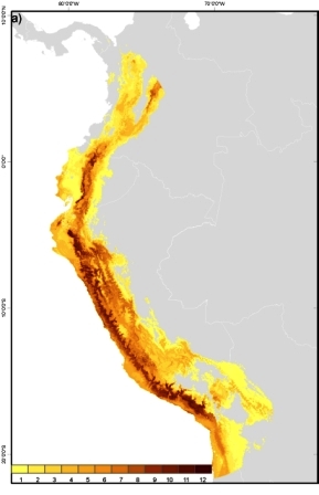
Tomato (Solanum lycopersicum L.) wild relatives potential richness map. This maps depicts the number of taxa that are potentially found per unit of area. Darker colours represent greater richness of the tomato genepool. (Map by N. P. Castañeda Álvarez/May 2012) |
Abstract
Since the completion of the original version of this chapter, even greater emphasis has been placed on the conservation and exploitation of the broader crop genepool and, as such, ecogeography remains a critical tool in formulating effective and efficient conservation strategies, although, increasingly, ecogeographic surveys are seen as an element within a more comprehensive systematic gap analysis (see chapter 41 in the 2011 version of these Technical Guidelines). However, ecogeographic techniques themselves have advanced significantly since the 1995 chapter on ecogeographic surveys, particularly in terms of information availability and management. Most notably, the affordability in terms of cost, timing and resolution of geographical information systems (GIS), as well as the improvement in (and lower costs for acquiring) hardware and software, now makes ecogeographic analysis a routine task for the agrobiodiversity conservationist. In this updated chapter on ecogeographic surveys, ecogeography itself is redefined and the relationship between ecogeography and gap analysis is reviewed. Progress in the current status of nine key areas is examined: (1) selection of target taxa, (2) ecogeographic database standards, (3) ecogeographic data availability, (4) collection methods for ecogeographic data, (5) on-line gazetteers, (6) threat assessment, (7) GIS analysis and prediction, (8) assessing the impact of climate change and (9) germplasm use. There have been significant advances in ecogeographic techniques in recent years, they remain critical to the conservation and utilization of plant genetic resources.
Introduction
The 1995 chapter starts with the statement that “plant collectors are like detectives: they gather and analyse clues in order to trace plants of interest.” This statement remains essentially as true today as it was in 1995 when the original text was compiled, although technically, today we may wish to stress more the tracing of genetic diversity within the broader crop genepool. Conservationists do not just look randomly for the diversity they are targeting; the planning and targeting of conservation is associated with careful preparation to identify where to sample germplasm, where to establish genetic reserves, and how precisely the resource will be conserved and later used. Essentially, ecogeographic surveys use historic provenance and population data as a basis for planning and targeting future conservation: past data are predictive. For example, given the requirement to conserve the perennial wild relative of garden peas Vavilovia formosa (Steven) Fed., we know that this species has historically always been found growing on limestone scree slopes above 2000 metres in Southwest Asia, so this is the habitat and location where we can expect to be able to collect germplasm for ex situ conservation or to conserve it in situ today. Although having made this simple point, it must be admitted that there are areas of the world that remain under-surveyed even today (such as eastern Turkey and the Democratic Republic of the Congo), and so past data are imperfect. But here we can use predictive modelling based on the available historic data to more effectively plan and implement conservation.
Soon after publication of the original chapter, it was clear that the definition of ecogeography needed to be amended; therefore, it is good to have the opportunity here to revise the definition. The first limitation was that the definition implied that only ecological, geographical and taxonomic information was used, but anyone that has undertaken an ecogeographic survey or study will know that knowledge of the pattern of genetic diversity for the target taxon is equally relevant to conservation planning. Given the conservation goal of maximizing genetic diversity, it could be argued that without full consideration of patterns of genetic diversity (where they are known), information based on ecological, geographical and taxonomic evidence could be misleading and could waste scarce conservation resources. The second problem with the definition is the separation of collection from broader conservation. It is now universally accepted that the application of in situ and ex situ techniques are necessary and complementary, the one providing (among other benefits) a security back-up for the other. The collation and analysis of ecogeographic data is an equally critical precursor for effective ex situ and in situ conservation, so both conservation strategies deserve equal weight in the definition. Therefore, the following revision of the definition of ecogeography is proposed:
Ecogeography is a process of gathering and synthesizing information on ecological, geographical, taxonomic and genetic diversity. The results are predictive and can be used to assist in the formulation of complementary in situ and ex situ conservation priorities.
When the 1995 text was prepared, there was already extensive literature on “gap analysis” (i.e., how to identify areas in which selected elements of biodiversity are underrepresented, e.g., see Margules 1989). This body of literature has continued to be extended (i.e., Balmford 2003; Brooks et al. 2004; Dietz and Czech 2005; Margules and Pressey 2000; Riemann and Ezcurra 2005). This literature was originally applied to indigenous forests, particularly on small islands rich in endemic species. However, Maxted et al. (2008) showed how the existing methodology might be adapted for more general conservation and proposed a specific methodology for the genetic gap analysis of crop wild relatives (CWR), which involves four steps: (a) identify priority taxa, (b) identify ecogeographic breadth and complementary hotspots using genetic diversity, distribution and environmental data, (c) match current in situ and ex situ conservation activities with the identified genetic diversity, ecogeographic breadth and complementary hotspots to identify the so-called conservation “gaps” and (d) formulate a revised in situ and ex situ conservation strategy. Gap analysis has rapidly established itself as the methodology for conservation planning (FAO 2009; Parra-Quijano et al. 2011; Ramírez-Villegas et al. 2010), not replacing ecogeography, but in reality subsuming ecogeography as an element within the gap analysis protocol. As such, ecogeographic surveys will continue to be routinely undertaken, but increasingly within a gap analysis context. Therefore, an additional chapter (Chapter 41 entitled “Gap Analysis: A Tool for Genetic Conservation”) has been added to these Guidelines, which reviews the gap analysis methodology. It should be seen as a sister chapter to read in conjunction with this chapter.
Current status
Although ecogeographic surveys are a necessary precursor to the conservation of both crop and wild plants, the increasing interest in the conservation and use of CWR diversity means that the techniques used to collate ecogeographic data have advanced significantly since 1995, most notably in the methods of data collation and subsequent analysis. The use of ecogeographic techniques for crop and wild-plant diversity was thoroughly reviewed by Guarino et al. (2006) and for crop wild relatives by Maxted and Guarino (2003). The following is a review of the major innovations since the original text was published in 1995, demonstrating the continuing value of ecogeographic techniques and the novel opportunities and challenges they offer for the conservationist.
Selection of target taxa
Any conservation action requires a clear target and, as mentioned in the 1995 text, this may be established in the project commission, but the recent creation of a global priority checklist of CWR taxa (Vincent et al., 2012; www.cwrdiversity.org/home/checklist) should assist conservation planning by having a pre-existing prioritizing list of priority taxa for the major and minor crops of the world. It is referred to as the Harlan and de Wet Global Priority Checklist to acknowledge the pioneering work of Harlan and de Wet (1971) in first proposing the Gene Pool (GP) concept to explain the relative value of species in their potential as gene donors for crop improvement. The database contains background information on 174 crop genepools and 1397 priority CWR species: those deemed priority CWRs as defined by their membership in GP1b or GP2, or Taxon Groups (TG) 1b, 2 or 3. There are also a limited number of GP3 and TG4 taxa included if they have previously been shown to be useful in breeding. The Gene Pool concept designated the crop itself as GP1a, while GP1b are the wild or weedy forms of the crop that cross easily with it. GP2 are secondary wild relatives (less closely related species from which gene transfer to the crop is possible but difficult using conventional breeding techniques), and GP3 are tertiary wild relatives (species from which gene transfer to the crop is impossible, or if possible, requires more advanced techniques, such as embryo rescue, somatic fusion or genetic engineering).
If the necessary crossability information is lacking, as it is for most crop genepools, then the taxon group concept (Maxted et al. 2006) can substitute for the genepool concept. The taxon group concept employs the taxonomic hierarchy as a proxy for taxon genetic relatedness and thus crossability, so TG1a is the crop, TG1b is the same species as the crop, TG2 is the same series or section as the crop, TG3 is the same subgenus as the crop, and TG4 is the same genus. The assumption is that the taxonomic classification is related to crossability, and if genepool and taxon group concepts are compared for those crop genepools where a genepool concept is known, this assumption seems well founded. The data recorded in the database for each crop include the associated published genepool concept or taxon group concept, complete with references, and confirmed and potential CWR taxa used in crop breeding and improvement. Then, for each taxon (including crop taxa) the following information is recorded: accepted name (standardized to the Plant List, www.theplantlist.org), taxonomic classification, common name, main synonyms, seed storage behaviour, geographic distribution, key herbaria holding specimens (derived from geographic distribution) and utilization data with references. It is expected that the checklist will be dynamic in that as new genepool or taxon group concepts are published, authors will be able to upload their concept to the online database and make it readily available to the user community. It will act as a guide to those establishing geographical and genepool CWR conservation priorities in individual countries or crops.
Ecogeographic database standards
Ecogeographic data, in part, describe the population location and, therefore, the ecology and environment where particular taxa may occur. It is common for these data to be organized under different standards, data structures and file formats, usually capturing different sorts of details. Thus, when merging ecogeographic information taken from different sources, attention is needed to combine similar information correctly and avoid combinations that might lead to mistakes or data loss.
Increasingly, global efforts to standardize biological information have promoted standards to improve the recording and exchange of data within databases. The Taxonomic Databases Working Group (TDWG) (www.tdwg.org) is one of the main initiatives for developing and promoting standards that enable the exchange of biological records. The current standard recommended by TDWG for biological records is the “Darwin Core” (http://rs.tdwg.org/dwc/index.htm). The standard “Access to Biological Collection Data” (http://wiki.tdwg.org/twiki/bin/view/ABCD/AbcdIntroduction) is also recommended; however, it does not comply with all the specifications of the working group. Alternative systems to organize, store and distribute biological information are also available. Botanical Records and Herbarium Management (BRAHMS) (http://dps.plants.ox.ac.uk/bol/brahms/Home/Index) is a well-known system, focused on herbaria, living collections and seed-bank data that enables users to manage, analyse and share their data.
Despite the relative diversity of standards available, interoperability between standards is becoming common, allowing data repositories to gather information and benefiting users who require access to biological records.
Online ecogeographic data availability
Perhaps one of the key changes between 1995 and today is the exponential growth of web-enabled ecogeographic datasets, most notably the Global Biodiversity Information Facility (GBIF) established in 2001 (http://data.gbif.org), which provides extensive access to global taxon nomenclature, taxon and accession distribution, conservation and environmental data. Established to encourage free and open access to biodiversity data via the internet and now encompassing a network of 57 countries and 47 organizations, GBIF promotes and facilitates the mobilization, access, discovery and use of information about the occurrence of organisms over time and across the planet. It facilitates the digitization and global dissemination of primary biodiversity data (e.g., data from natural history collections, libraries and databases). GBIF taxon searches can be limited to the country or countries of interest, or data can be downloaded and the necessary records extracted. To access data via GBIF (http://aegro.jki.bund.de/aegro/index.php?id=195):
-
Use the search facility to find data on your taxon of interest.
-
When you click on the taxon link provided, you will be asked to accept the terms of the GBIF user license agreement. Read the terms and then click on “Accept terms”.
-
You will then be provided with a number of links to data related to your taxon. Follow these links to find the information needed. For example, click on “occurrences” to find a list of recorded occurrences of the taxon (note that the map function will not show distribution data unless there are coordinates available).
-
To save a list of the occurrences, you can download the results in different table formats (i.e., as an MS Excel spreadsheet or as tab- or comma-delimited text).
-
Before you download the data, you can limit the fields included by unchecking the fields that are not needed. However, it is advisable to download all data, then delete or hide those fields that are not needed, in case the data might be of use at a later date.
GBIF has rapidly become the largest web-enabled supplier of nomenclatural, distribution, conservation and environmental data, drawing information from a growing global network of natural history collections and associated agencies.
 |
|
|
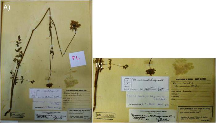
Example of specimen and label for digitization from Herbário João de Carvalho e Vasconcellos, Instituto Superior de Agronomia, Lisbon, Portugal (Photos: N. P. Castañeda Álvarez) |
The plant information accessible via GBIF is primarily derived from digitized herbarium or field records. There are other initiatives being developed to provide access to herbarium specimens, as well as national programs that are digitizing their collections and making the data available via the internet (table 14.1). Therefore, once the priority list of herbaria and gene banks that are likely to contain the necessary CWR collections have been identified, the herbarium and gene bank websites should be visited to see if the required data are online, which would further reduce the need and expense of visits to herbaria and gene banks.
Table 14.1: Data on Herbarium and National Collections Being Digitized for Internet Access
|
|
|
|
||
|
JSTOR Plant Science |
images of specimens from 155 institutions |
|||
|
|
||||
|
GENESYS |
a global portal to germplasm accession holdings of plant genetic resources for food and agriculture |
|||
|
European Plant Genetic Resources Search Catalogue (EURISCO) |
||||
|
System-wide Information Network for Genetic Resources (SINGER) |
||||
|
Genetic Resources Information Network of the United States Department of Agriculture (GRIN) |
||||
|
|
||||
|
|
||||
|
|
||||
|
|
||||
|
Russia |
AgroAtlas |
|||
|
Brazil |
CRIA |
|||
|
Japan |
NIAS |
|||
|
Mexico |
||||
|
|
||||
|
Harold and Adele Lieberman Germplasm Bank (cereals) |
||||
|
Manchester Museum |
||||
|
Millennium Seed Bank, Kew |
www.kew.org/science-conservation/save-seed-prosper/millennium-seed-bank/index.htm |
|||
|
National History Museum, UK |
||||
|
Royal Botanic Gardens Kew |
||||
|
Royal Botanical Garden of Edinburgh |
||||
|
SolanaceaeSource |
www.nhm.ac.uk/research-curation/research/projects/solanaceaesource |
|||
|
United States Virtual Herbarium |
||||
|
Virtual Australian Herbarium |
http://plantnet.rbgsyd.nsw.gov.au/HISCOM/Virtualherb/virtualherbarium.html#Virtual |
|||
One consequence of the recent efforts to digitize specimen and accession records and to make them available through multiple web-enabled databases and portals is that the same information may be duplicated in several sites. Care should be taken to eliminate duplicates if they are likely to bias subsequent analyses and give a false impression of the actual current conservation status of target taxa.
As shown in figure 14.1, not every specimen’s passport information from a particular herbarium is available through the internet; therefore, it is necessary to arrange visits to herbaria to query the local databases and also to get information for specimens that are not available through any database.
|
Figure 14.1: Availability of specimen information from the world’s main herbaria through GBIF |
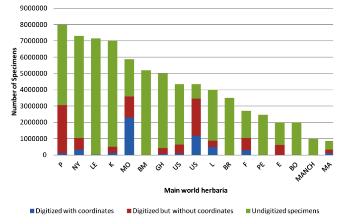 |
|
Note: P = Muséum National d'Histoire Naturelle, Paris; NY = New York Botanical Garden, New York; LE = Karmarov Institute, St Petersburg; K = Royal Botanic Gardens, Kew; MO = Missouri Botanical Garden, St Louis; GH = Harvard University, Cambridge, MA; US = Smithsonian Institution, Washington DC; L = Nationaal Herbarium Nederland, Leiden; BR = National Botanic Garden of Belgium, Meise; F = Field Museum of Natural History, Chicago; PE = Institute of Botany, Chinese Academy of Sciences, Beijing; E = Royal Botanic Garden, Edinburgh; BO = Herbarium Bogoriense, Cibinong; MANCH = University of Manchester, Manchester; MA = Real Jardín Botánico, Madrid. |
Methods for collecting ecogeographic data
|
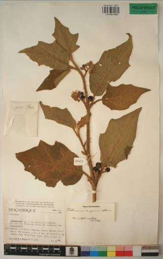
Figure 14.2: Example of the photographic approach for a specimen of Solanum anguivi |
|
 |
|
|
Source: Courtesy of Instituto de Investigação Científica Tropical–Jardim Botânico Tropical, Lisbon, Portugal. |
In the 1995 text, it was largely assumed that the way to collate ecogeographic data was for the conservationist to select priority herbaria or gene banks, visit the priority institutions, select specimens or accessions (largely on the basis of quality of ecogeographic data) and then type the selected specimen or accession passport data into a computer. This is still likely to be the most commonly used approach. However, currently this is not the only method that can be employed; the project on Adapting Agriculture to Climate Change, led by the Global Crop Diversity Trust (Guarino and Lobell 2011), is using an approach that is based more on photography (see figure 14.2). This involves visiting the priority herbaria, photographing the selected specimens, and then, back at base, working out the latitude and longitude necessary for GIS analysis (see Annex A for more detailed instructions). This approach has the obvious advantage of being relatively quick, therefore reducing the time the conservationist needs to spend at the host herbarium, and it provides a permanent image of the specimen, which can be checked if the identification is thought to be incorrect. It also means that specimen identification in the herbarium is not as critical because the image may later be seen and validated by an expert.
The Adapting Agriculture to Climate Change project has also defined the minimum threshold at 20 specimens, to produce a reliable distribution model representing the potential geographic areas in which the species might be found (Hernandez et al. 2006; Pearson et al. 2007; Wisz et al. 2008). Further, the project has extended the list of ecogeographic data that can be obtained from herbarium specimens (see Annex B).
On-line gazetteers
Ecogeographic data gathered through visits to herbaria, exchanges with other researchers, or querying online databases generates lists of locations where a certain specimen has been reported and/or collected. Recent collections might also include precise coordinates taken with GPS. When only a description of the locality is available, it is necessary to use some form of gazetteer to establish the location more precisely, a process that is sometimes called georeferencing.
Choosing which of the available strategies to use depends on the time and resources available. Manual methods (which use book gazetteers that list locations with latitude and longitude, and detailed maps) are still useful, particularly for those who are familiar with the localities where the specimen was originally collected. It is recommended that this strategy be applied to small datasets (i.e., fewer than 100 records) because it is very time consuming. Increasingly, for larger datasets, reliable online services, such as that of the National Geospatial-Intelligence Agency (NGA) (http://earth-info.nga.mil/gns/html), are used. The NGA provides the NGA GEOnet Names Server (GNS), which allows the user to retrieve information based on administrative and locality details. An advantage of this service is that it provides information about the features that are present in the area (e.g., rivers, populated areas, administrative divisions).
More-automated services are also available through the internet. However, care needs to be taken when using these; some are not always available because of lack of maintenance of servers, services that are no longer free, etc. They require data to be submitted in specific formats, and the percentage of locations found is usually low (only 10% to 15%). Biogeomancer (http://bg.berkeley.edu) is a widely known service aiming to improve the quality and quantity of biodiversity data represented in maps. It has an option to georeference records by batch, but first you are required to register on their site. The main advantage of Biogeomancer is that it calculates the uncertainty of each estimated coordinate, allowing the user to decide whether it is useful for his/her analysis. Although not implemented yet, the Google Geocoding API (https://developers.google.com/maps/documentation/geocoding) might also be a tool of interest for georeferencing biological data because of the search algorithms supported by Google and also the ease of creating personalized routines through the API.
Threat assessment
In recent years there have been several initiatives to conserve CWR diversity, most notably the project on Adapting Agriculture to Climate Change (Guarino and Lobell 2011). While this will result in more systematic complementary conservation of CWR diversity in time, the sheer numbers of CWR taxa make comprehensive CWR conservation unlikely. Conservationists will continue to need to prioritize and select which taxa to conserve. One commonly used means of doing this is relative threat.
It is recognized worldwide that biodiversity is currently under severe threat from a range of deleterious factors, such as habitat destruction, degradation and fragmentation, overexploitation, introduction of exotic species, and changes in agricultural practices and land use. However, the predicted impact of climate change is likely to be more catastrophic in terms of the loss of both species and infraspecific genetic diversity. Globally, Hilton-Taylor et al. (2008) estimate that since the year 1500, 115 plant species have become extinct or extinct in the wild, a further 8457 plant species are at risk of extinction, and approximately two-thirds of assessed plants are currently threatened. Further, climate change is predicted to increase average temperatures by 2°C to 4°C in Europe over the next 50 years, which will cause considerable changes in regional and seasonal patterns of precipitation (IPCC 2007). This will have a direct impact on the natural reproductive cycles and distribution of wild plant species, and is predicted to result in a 27% to 42% loss of plant species in Europe by 2080 (Thuiller et al. 2005) and a 60% loss of mountain plant species by 2100 (EEA 2009). Although it is difficult to quantify the loss of genetic diversity within species, it is likely to be very much greater than the loss of species themselves, given that most of the species that remain extant will suffer some loss of genetic diversity (Maxted 2003; Maxted et al. 1997a). It can be argued that CWR species are particularly threatened by climate change because many are associated with disturbed habitats (Hopkins and Maxted 2010) and these habitats are particularly threatened by climate change (Hopkins et al. 2007).
In the face of this level of threat, it is perhaps inevitable that the relative threat to a taxon will be used as a means of prioritizing plant genetic resources for conservation and that threat assessment will either be associated with or become an element of an ecogeographic survey, particularly given that the necessary data required for threat assessment are commonly generated during an ecogeographic survey. For general threat assessment and prioritization of biodiversity, the standardized system of applying the IUCN Red List categories (IUCN 2001) is commonly used. The IUCN threat assessment is data-driven on the basis of different criteria under which a taxon may be listed, each with distinct data requirements. However, the IUCN criteria assess the entire taxon, commonly at species level, and conservation of the range of genetic diversity within taxa or landraces is not easily considered. Various authors have used the IUCN Red List ethos to propose a set of categories and criteria for landrace threat assessment (Joshi et al. 2004; Porfiri et al. 2009).
Even with the limitations of assessing genetic diversity using the IUCN Red List categories, the technique is useful in distinguishing species-level priorities. The first extensive IUCN Red List assessment of CWR diversity has recently been published for European species (Bilz et al. 2011; Kell et al. 2012). In total, 571 native European CWR of high-priority human and animal food-crop species were assessed: 313 (55%) were assessed as Least Concern, 166 (29%) as Data Deficient, 26 (5%) as Near Threatened, 22 (4%) as Vulnerable, 25 (4%) as Endangered and 19 (3%) as Critically Endangered. All assessments have been published on the IUCN Red List website (www.iucnredlist.org). The most common threatening factors recorded were intensive “livestock farming and ranching”, increasing “tourism and recreation areas” and development of “housing and urban areas”. Nearly half of the CWR species had at least one accession conserved ex situ but virtually none were actively conserved in situ in protected areas. It would be useful if this initiative were repeated in other regions, as readily available Red List assessments would facilitate the ecogeographic process.
GIS analysis and prediction
Geographic information systems (GIS) have proved to be very flexible tools with applications in countless areas, including business, government, the sciences and nongovernmental organizations (ESRI 2012). The use of GIS for agriculture, ecology, biogeography and studies of natural resources has helped us to better understand patterns and relationships between different elements of nature. In particular, GIS has been used in studies of plant genetic resources to identify areas of high diversity (Maxted et al. 2004; Ocampo et al. 2007; Scheldeman et al. 2007; and chapter 15/16 in these updated Guidelines), species requiring further conservation (Dulloo et al. 1999; Jarvis et al. 2003), potential areas to collect germplasm (Ferguson et al. 1998; Jarvis et al. 2005; Parra-Quijano et al., 2011; Ramírez-Villegas et al. 2010), suitable areas for in situ conservation (Draper et al. 2003; Maxted 1995; Peters et al. 2005) and levels of threats affecting plant species (Jarvis et al. 2008), as well as creating informative compilations such as atlases (Azurdia et al. 2011; Hijmans et al. 2002).
Species distribution modelling (SDM) algorithms are tools frequently used in studies of plant genetic resources because they allow the prediction of areas that meet the environmental conditions required by a particular species. SDM inputs differ by algorithm (table 14.2).
Table 14.2: List of Algorithms for Species Distribution Modelling
|
Modelling algorithm |
Type of input required |
Software source |
|
Maxent (Phillips et al. 2006) |
Presence and absence |
|
|
Bioclim (Nix 1986) |
Presence data |
|
|
DOMAIN (Carpenter et al. 1993) |
Presence data |
|
|
Artificial Neural Networks (ANN) |
Presence data |
|
|
Ecological-Niche Factor Analysis – ENFA- |
Presence data |
|
|
Genetic Algorithm for Rule Set Production –GARP- (Stockwell and Noble 1992) |
Presence and absence data |
|
|
HABITAT (Walker and Cocks 1991) |
Presence data |
|
|
Generalized Linear Model-GLM- |
Presence and absence data |
R: package “dismo”, function “glm” |
|
Generalized Additive Model (GAM) |
Presence and absence |
R: package “mgcv” |
|
Mahalanobis Distance (MD) |
Presence data |
|
|
Classification Tree Analysis (CTA) |
R: package “BIOMOD” |
|
|
Surface Range Envelope (SRE) |
R: package “BIOMOD” |
|
|
Generalized Boosting Model (GBM) |
Presence and absence data |
R: package “BIOMOD” |
|
Breiman and Cutler’s random forest for classification and regression (RF) |
R: package “BIOMOD” |
|
|
Flexible Discriminant Analysis (FDA) |
R: package “BIOMOD” |
|
|
Multiple Adaptive Regression Splines (MARS) |
Presence and absence data |
R: package “BIOMOD” |
SDM algorithms require inputs as presence (and absence) data and environmental layers. Sources of environmental layers at the global scale are Worldclim (www.worldclim.org), which offers precipitation and temperature layers (Hijmans et al. 2005), SRTM-CIAT (http://srtm.csi.cgiar.org), containing digital elevation data, and Global Land Cover (http://glcf.umiacs.umd.edu).
Assessing the impact of climate change
Climate change is a global concern, as growing evidence demonstrates that it is already happening and future scenarios calculate that its effects are likely to have a drastic impact on life on earth (IPCC 2001, 2007). Agrobiodiversity is not an exception; it also is likely to suffer genetic erosion and extinction, but crop landrace and CWR diversity are expected to offer sources of traits to adapt crops to climate change (Farooq and El-Azam 2004; Hajjar and Hodgkin 2007; Maxted et al. 1997). However, other taxa might not respond adequately to such effects of climate change as floods, drought, heat and changes in precipitation patterns.
Analysis based on algorithms that model species distribution and on global circulation models (GCMs) permit us to produce estimates on how climate change will affect the environmental conditions where species are found. One such study is by Jarvis et al. (2008), which evaluated the predicted impact of climate change by 2055 on the CWR of groundnut (Arachis), potato (Solanum tuberosum) and cowpea (Vigna), finding that 16% to 22% of all species modelled (316) are at risk of extinction, while a significant number of species might lose more than 50% of their geographic coverage. Perhaps also of concern was the finding that the predicted impact of climate change varied significantly between crops: they found that 24 to 31 (of the 51) Arachis species were projected to become extinct and their distribution area reduced by 85% to 94% over the next 50 years, while Vigna species were predicted to lose only zero to two of the 48 species. This demonstrates the importance of assessing the impact of climate change for all landraces or CWR taxa in threatened areas.
Links to germplasm use
As noted above, in recent years there have been several initiatives to systematically conserve CWR diversity; however, the goal of genetic conservation is not just to maximize the genetic diversity conserved but also to promote its exploitation, and users are more likely to exploit diversity if it is easily accessible and meets their requirements. Two consequences follow from this statement: first, although the two conservation strategies are complementary and should be applied together for any genepool, they are not of equal value in terms of their application for the user. It is well established that users are more likely to exploit ex situ conserved resources because of the ease of access; the greater likelihood that characterization, evaluation and pre-breeding has been undertaken; the fact that in situ conserved resources are likely to be more remote to the user; and seed will only be available for part of the growing cycle. As such, there is a utilization argument for always ensuring that in situ conserved material is also duplicated ex situ. Ex situ conservation is more than a mere safety back-up of in situ conservation.
Second, with limited resources for any form of active conservation, there will always be a need to prioritize target taxa, and if one of the reasons for conservation is utilization, then it can be argued that the conservationist should have a clear idea what the user community requires. Therefore, it can be argued that if it has not already been considered as part of the conservation commissioning process, an additional element of the ecogeographic survey would be a review of the user community’s requirements. And by “user community”, we would mean breeders attempting to address climate change mitigation or changing consumer demands, landscape restorers trying match taxa for planting in a particular locality, or disaster relief agencies or individual farmers trying to replace locally adapted crop landraces. FAO (2009) emphasizes that “Considerable opportunities exist for strengthening cooperation among those involved in the conservation and sustainable use of PGRFA, at all stages of the seed and food chain. Stronger links are needed, especially between plant breeders and those involved in the seed system, as well as between the public and private sectors.” An analysis of user requirements would ensure greater use of conserved material, ensure that conserved germplasm is more than a museum exhibit, secure the long-term future of the conservation action itself and, finally, create opportunities to develop new partnerships that bridge the gap between the conservation and use of CWR and landraces.
Future challenges/needs/gaps
It may be that, in time, ecogeographic surveys will be subsumed as a component of the more encompassing and structured gap analysis approach to conservation planning, but whether this is the case or not, the collation, analysis and use of ecogeographic data will remain a key facet of conservation planning.
It seems likely that, with time, the limited availability of passport data for ecogeographic analysis will diminish as more and more natural history collections are digitized and web-enabled, although this is likely to remain limited in smaller herbaria and gene banks where resources are scarce. The problem may be that the analysis of the vast ecogeographic datasets that are available, with such large and complex datasets, will require a new generation of analysis programs, in terms of both multivariate statistic and GIS capabilities. A key question also remains of how much data do we need to analyse in order to obtain a significant answer? How many herbarium records is enough? In the 1995 text, the authors concluded that “There is no specific answer to this question.” But, upon reflection, it now seems that more concrete advice would be helpful. As noted above, for the project on Adapting Agriculture to Climate Change, it is recommended that the passport data from a minimum of 20 specimens per species be included. However, a recent study by Feeley and Silman (2011a) concluded that significantly larger sample sizes (of 75 to 100) are required to accurately map species ranges, although they also note that only around 5% of tropical plant species are represented by more than 20 specimens (Feeley and Silman 2011b). The project on Adapting Agriculture to Climate Change could provide a practical answer to this question.
The ground-breaking paper published by Jarvis et al. (2008) evaluated the predicted impact of climate change on three crop genepools: groundnut (Arachis), potato (Solanum tuberosum) and cowpea (Vigna). They showed that all species modelled are at risk of extinction and some may lose more than 50% of their geographic coverage. An interesting facet of this analysis was that the genepools were predicted to respond significantly differently to climate change. What about a broader survey of crop genepools? We now have a global priority list of 1397 CWR species. How is each of them likely to respond and how will their vulnerability affect conservation priorities? Given the growing concern over the impact of climate change and food security, surely a broader survey is an urgent priority.
Einstein once commented that “God does not play dice” in relation to the formation of the universe. It can be equally argued that neither should conservationists. No conservationists would get into a land cruiser, drive and hope to bump into the plant they hope to conserve. Ecogeography is at the heart of all conservation planning; however, ecogeographic surveys are still too often commissioned on an ad hoc basis. It can be argued that adopting a more strategic approach to global, regional and national conservation planning would not only be effective but would also save scarce conservation resources.
Conclusions
There have been significant advances in the techniques associated with ecogeographic surveys in recent years, particularly in data capture and data analysis, but there are likely to be additional advances in the next few years. There will be a need for a new generation of multivariate statistical and GIS techniques to enable the potentially vast and complex datasets that are likely to become available for routine use in planning conservation activities.
Back to list of chapters on collecting
References and further reading
Azurdia C, Williams K, Williams D, Van Damme A, Jarvis A, Castaño S. 2011. Atlas of Guatemalan Crop Wild Relatives. Available online (accessed 10 June 2012): www.ars.usda.gov/ba/atlascwrguatemala.
Balmford A. 2003. Conservation planning in the real world: South Africa shows the way. Trends in Ecology and Evolution 18:435–438.
Bilz M, Kell SP, Maxted N, Lansdown RV. 2011. European Red List of Vascular Plants. Publications Office of the European Union, Luxembourg. Available online (accessed 18 June 2012): http://ec.europa.eu/environment/nature/conservation/species/redlist/downloads/European_vascular_plants.pdf
Brooks TM, Bakarr MI, Boucher T, da Fonseca GAB, Hilton-Taylor C, Hoekstra JM. 2004. Coverage provided by the global PA system: Is it enough? Bioscience 54(12):1081–1091.
Carpenter G, Gillison N, Winter J. 1993. DOMAIN: A flexible modeling procedure for mapping potential distributions of plants and animals. Biodiversity and conservation 2(6): 667–680.
Dietz RW, Czech B. 2005. Conservation deficits for the continental United States: An ecosystem gap analysis. Conservation Biology 19:1478–1487.
Draper D, Rosselló-Graell A, García C, Tauleigne Gomes C, Sérgio C. 2003. Application of GIS in plant conservation programmes in Portugal. Biological Conservation 113(3):337–349.
Dulloo ME, Guarino L, Engelmann F, Maxted N, Newbury HJ, Attere F, Ford-Lloyd BV. 1999. Complementary conservation strategies for the genus Coffea with special reference to the Mascarene Islands. Genetic Resources and Crop Evolution 45:565–579.
EEA. 2007. European Nature Information System (EUNIS). European Environment Agency, Copenhagen. Available online (accessed 10 June 2012): http://eunis.eea.europa.eu/index.jsp.
EEA. 2009. Distribution of Plant Species (CLIM 022). European Environment Agency, Copenhagen.
ESRI. 2012. What is GIS? Available online (accessed 10 June 2012): www.esri.com/what-is-gis/who-uses-gis.html.
FAO. 2009. Second Report on the State of the World’s Plant Genetic Resources for Food and Agriculture. Food and Agriculture Organization of the United Nations, Rome.
Farooq S, El-Azam F. 2004. Co-Existence of salt and drought tolerance in Triticeae. Hereditas 135(2–3): 205–210.
Feeley KJ, Silman MR. 2011a. The data void in modelling current and future distribution of tropical species. Environmental Conservation 24:733–740.
Feely KJ, Silman MR. 2011. Keep collecting: accurate species distribution modelling requires more collections than previously thought. Diversity and Distributions (2011):1–9. Available online (accessed 6 October 2011): www.wfu.edu/~silmanmr/labpage/publications/divdist.keep.collecting.2011.pdf.
Ferguson ME, Ford-Lloyd BV, Robertson LD, Maxted N, Newbury HJ. 1998. Mapping the geographical distribution of genetic variation in the genus Lens for the enhanced conservation of plant genetic diversity. Molecular Ecology 7:1743–1755.
GBIF. n.d. Global Biodiversity Information Facility – data portal. Available online (accessed 10 June 2012): http://data.gbif.org.
Guarino L, Lobell DB. 2011. A walk on the wild side. Nature Climate Change 1:374–375.
Guarino L, Maxted N, Chiwona EA. 2006. A methodological model for ecogeographic surveys of crops. IPGRI Technical Bulletin No. 9. International Plant Genetic Resources Institute, Rome.
Hajjar R, Hodgkin T. 2007. The use of wild relatives in crop improvement: A survey of developments over the last 20 years. Euphytica 156:1–13.
Harlan JR, de Wet JMJ. 1971. Towards a rational classification of cultivated plants. Taxon 20:509–517.
Hernandez PA, Graham CH, Master LL, Albert DL. 2006. The effect of sample size and species characteristics on performance of different species distribution modeling methods. Ecography 29(5):773–785. Available online (accessed 6 October 2011): http://onlinelibrary.wiley.com/doi/10.1111/j.0906-7590.2006.04700.x/abstract.
Hijmans R, Spooner D, Salas A, Guarino L, de La Cruz J. 2002. Atlas of Wild Potatoes. Systematic and Ecogeographic Studies on Crop Genepools 10. International Plant Genetic Resources Institute, Rome.
Hijmans RJ, Cameron SE, Parra JL, Jones PG, Jarvis A. 2005a. Very high resolution interpolated climate surfaces for global land areas. International Journal of Climatology 25:1965–1978. Available online (accessed 6 October 2011): www.worldclim.org/worldclim_IJC.pdf.
Hilton-Taylor C, Pollock CM, Chanson JS, Butchart SHM, Oldfield TEE, Katariya V. 2008. State of the world’s species. . In: Vié J-C, Hilton-Taylor C, Stuart SN, editors. Wildlife in a Changing World: An Analysis of the 2008 IUCN Red List of Threatened Species. International Union for Conservation of Nature, Gland, Switzerland. pp. 15–42.
Hirzel AH, Hausser J, Chessel D, Perrin N. 2002. Ecological-niche factor analysis: How to compute habitat-suitability maps without absence data? Ecology 83:2007–2036.
Hopkins J, Maxted N. 2010. Crop Wild Relatives: Plant Genetic Conservation for Food Security. Natural England, Peterborough, UK.
Hopkins JJ, Allison HM, Walmsley CA, Gaywood M, Thurgate G. 2007. Conserving Biodiversity in a Changing Climate: Guidance on Building Capacity to Adapt. Department for Environment, Food and Rural Affairs, London
Hunter D, Heywood V. 2011. Crop Wild Relatives: A Manual of In Situ Conservation. Earthscan, London.
IPCC. 2001. IPCC Third Assessment Report: Climate Change 2001 (TAR). Intergovernmental Panel on Climate Change, Geneva.
IPCC. 2007. Fourth Assessment Report: Climate Change 2007. Synthesis Report. Intergovernmental Panel on Climate Change, Geneva.
IUCN. 2001. IUCN Red List Categories and Criteria: Version 3.1. IUCN Species Survival Commission. International Union for Conservation of Nature and Natural Resources, Gland, Switzerland and Cambridge, UK. Available online (accessed 10 June 2012): www.iucnredlist.org/documents/redlist_cats_crit_en.pdf.
Jarvis A, Lane A, Hijmans RJ. 2008. The effect of climate change on crop wild relatives. Agriculture, Ecosystems and Environment 126:13–23. Available online (accessed 6 October 2011): www.abcic.org/index.php?option=com_docman&task=doc_download&gid=9&Itemid=77.
Jarvis A, Ferguson ME, Williams DE, Guarino L, Jones PG, Stalker HT, Valls JFM, Pittman RN, Simpson CE, Bramel P. 2003. Biogeography of wild Arachis: assessing conservation status and setting future priorities. Crop Science 43(3):1100–1108. Available online (accessed 6 October 2011): http://ciat-library.ciat.cgiar.org/Articulos_Ciat/ajarvis.pdf.
Jarvis A, Williams K, Williams D, Guarino L, Caballero P, Mottram G. 2005. Use of GIS for optimizing a collecting mission of rare wild pepper (Capsicum flexuosum Sendtn.) in Paraguay. Genetic Resources and Crop Evolution 52(6):671–682. Available online (accessed 18 February 2012): http://ddr.nal.usda.gov/handle/10113/18374.
Joshi BK, Upadhyay MP, Gauchan D, Sthapit BR, Joshi KD. 2004. Red listing of agricultural crop species, varieties and landraces. Nepal Agricultural Research Journal 5:73–80.
Kell SP, Maxted N, Bilz M. 2012. European crop wild relative threat assessment: Knowledge gained and lessons learnt. In: Maxted N, Dulloo ME, Ford-Lloyd BV, Frese L, Iriondo JM, Pinheiro de Carvalho MAA, editors. Agrobiodiversity Conservation: Securing the Diversity of Crop Wild Relatives and Landraces. CAB International, Wallingford. pp. 218–242.
Margules CR. 1989. Introduction to some Australian developments in conservation evaluation. Biological Conservation 50:1–11.
Margules CR, Pressey RL. 2000. Systematic conservation planning. Nature 405(6873):243–253.
Margules CR, Nicholls AO, Pressey PL. 1988. Selecting networks of reserves to maximize biological diversity. Biological Conservation 43:63–76.
Maxted N. 1995. An Ecogeographic Study of Vicia Subgenus Vicia. Systematic and Ecogeographic Studies in Crop Genepools 8. International Board for Plant Genetic Resources, Rome.
Maxted, N. 2003. Conserving the genetic resources of crop wild relatives in European protected areas. Biological Conservation 113(3): 411–417.
Maxted N, Guarino L. 2003. Planning plant genetic conservation. In: Smith RD, Dickie JB, Linington SH, Pritchard HW, Probert RJ, editors. Seed Conservation: Turning Science into Practice. Royal Botanic Gardens, Kew. pp 37–78.
Maxted N, Hawkes JG, Guarino L, Sawkins M. 1997a. Towards the selection of taxa for plant genetic conservation. Genetic Resources and Crop Evolution 44:337–348.
Maxted N, Ford-Lloyd BV, Hawkes JG, editors. 1997b. Plant Genetic Conservation: The In Situ Approach. Chapman & Hall, London.
Maxted N, Mabuza-Dlamini P, Moss H, Padulosi S, Jarvis A, Guarino L. 2004. An Ecogeographic Survey: African Vigna. Systematic and Ecogeographic Studies of Crop Genepools 10. International Board for Plant Genetic Resources, Rome.
Maxted N, Ford-Lloyd BV, Jury SL, Kell SP, Scholten MA. 2006. Towards a definition of a crop wild relative. Biodiversity and Conservation 15(8):2673–2685.
Maxted N, Dulloo E, Ford-Lloyd BV, Iriondo J, Jarvis A. 2008. Genetic gap analysis: A tool for more effective genetic conservation assessment. Diversity and Distributions 14:1018–1030.
Moore JD, Kell SP, Iriondo JM, Ford-Lloyd BV, Maxted N. 2008. CWRML: Representing crop wild relative conservation and use data in XML. BMC Bioinformatics 9: 116. DOI:10.1186/1471-2105-9-116.
Nix HA. 1986. A Biogeographic Analysis of Australian Elapid Snakes. Atlas of Elapid Snakes of Australia. Australian Flora and Fauna Series Number 7. Australian Government Publishing Service, Canberra.
Ocampo J, d’Eeckenbrugge C, Restrepo M, Jarvis A, Salazar M, Caetano C. 2007. Diversity of Colombian Passifloraceae: Biogeography and an updated list for conservation. Biota Colombiana 8(1):1–45.
Parra-Quijano M, Iriondo JM, Torres E. 2011. Improving representativeness of genebank collections through species distribution models, gap analysis and ecogeographical maps. Biodiversiy and Conservation 21:79–96.
Pearson R, Raxworthy C, Nakamura M, Townsend Peterson A. 2007. Predicting species distributions from small numbers of occurrence records: A test case using cryptic geckos in Madagascar. Journal of Biogeography 34(1): 102–117.
Peters M, Hyman G, Jones P. 2005. Identifying areas for field conservation of forages in Latin American disturbed environments. Ecology and Society 10(1). Available online (accessed 10 June 2012): www.ecologyandsociety.org/vol10/iss1/art1.
Phillips SJ, Anderson RP, Schapire RE. 2006. Maximum entropy modeling of species geographic distributions. Ecological Modelling 190:231–259. Available online (accessed 6 October 2011): www.cs.princeton.edu/~schapire/papers/ecolmod.pdf.
Porfiri O, Costanza MT, Negri V. 2009. Landrace inventories in Italy and the Lazio region: Case study. In: Veteläinen M, Negri V, Maxted N, editors. European Landraces: On-Farm Conservation, Management and Use. Bioversity Technical Bulletin 15. Bioversity International, Rome. pp. 117–123.
Ramírez-Villegas J, Khoury C, Jarvis A, Debouck DG, Guarino L. 2010. A gap analysis methodology for collecting crop genepools: a case study with Phaseolus beans. PLoS ONE 5(10):e13497. Available online (accessed 28 October 2011): http://www.plosone.org/article/info%3Adoi%2F10.1371%2Fjournal.pone.0013497.
Riemann H, Ezcurra E. 2005. Plant endemism and natural PAs in the peninsula of Baja California, Mexico. Biological Conservation 122:141–150.
Scheldeman X, Willemen L, d’Eeckenbrugge C, Romeijn-Peeters E, Restrepo M, Romero J, Jiménez D, Lobo M, Medina C, Reyes C, Rodríguez D, Ocampo JA, Van Damme P, Goetgebeur P. 2007. Distribution, diversity and environmental adaptation to highland papayas (Vasconcellea spp.) in tropical and subtropical America. Biodiversity Conservation 16:1867–1884.
Stockwell DR, Noble I. 1992. Induction of sets of rules from animal distribution data: A robust and informative method of analysis. Mathematics and Computers in Simulation 33:385–390.
Thiers B. n.d. Index Herbariorum: A Global Directory of Public Herbaria and Associated Staff. New York Botanical Garden's Virtual Herbarium, New York. Available online (accessed 10 June 2012): http://sweetgum.nybg.org/ih
Thuiller W, Lavorel S, Araújo MB, Sykes MT, Prentice IC. 2005. Climate change threats to plant diversity in Europe. Proceedings of the National Academy of Sciences 102(23):8245–8250.
Vincent HA, Wiersema J, Dobbie SL, Kell SP, Fielder H, Castañeda Alvarez NP, Guarino L, Eastwood R, Leόn B, Maxted N. 2012. A prioritised crop wild relative inventory to help underpin global food security. Science (in preparation).
Walker PA, Cocks KD. 1991. HABITAT: A procedure for modelling a disjoint environmental envelope for a plant or animal species. Global Ecology and Biogeography Letters 1:108–118.
Wisz M, Hijmans R, Li J, Peterson AT, Graham CH, Guisan A, NCEAS Predicting Species Distributions Working Group. 2008. Effects of sample size on the performance of species distribution models. Diversity and Distributions 14:763–773.
Access to Biological Collection Data, standard: http://wiki.tdwg.org/twiki/bin/view/ABCD/AbcdIntroduction
AgroAtlas (Russia): www.agroatlas.ru
Artificial Neural Networks (ANN): http://openmodeller.sourceforge.net
Bioclim (Nix 1986): http://diva-gis.org
Biogeomancer: http://bg.berkeley.edu
Botanic Garden Conservation International (BGCI) database: www.bgci.org/plant_search.php
Botanical Records and Herbarium Management (BRAHMS): http://dps.plants.ox.ac.uk/bol/brahms/Home/Index
CRIA (Brazil): www.cria.org.br
Darwin Core, standard: http://rs.tdwg.org/dwc/index.htm
DOMAIN (Carpenter et al. 1993): http://diva-gis.org
Ecological-Niche Factor Analysis (ENFA) (Hirzel et al. 2002): www2.unil.ch/biomapper
ENSCONET: http://enscobase.maich.gr
European Plant Genetic Resources Search Catalogue (EURISCO): http://eurisco.ecpgr.org/nc/home_page.html
GENESYS: www.genesys-pgr.org
Genetic Algorithm for Rule Set Production (GARP) (Stockwell and Noble 1992): www.nhm.ku.edu/desktopgarp
Genetic Resources Information Network of the United States Department of Agriculture (GRIN): www.ars-grin.gov/npgs/searchgrin.html
Global Biodiversity Information Facility (GBIF): http://data.gbif.org
Global Land Cover: http://glcf.umiacs.umd.edu
Global priority checklist (The Harlan and de Wet Crop Wild Relative Checklist): www.cwrdiversity.org/home/checklist
Google Geocoding API: https://developers.google.com/maps/documentation/geocoding
Harold and Adele Lieberman Germplasm Bank (cereals): www.tau.ac.il/lifesci/units/ICCI/genebank1.html
Index Herbariorum: http://sciweb.nybg.org/science2/IndexHerbariorum.asp
IUCN Red List: www.iucnredlist.org
JSTOR Plant Science (images of specimens from 155 institutions): http://plants.jstor.org
Mahalanobis Distance (MD): www.jennessent.com/arcview/mahalanobis_grids.htm
Manchester Museum: http://emu.man.ac.uk/mmcustom/BotQuery.php
Maxent (Phillips et al. 2006): www.cs.princeton.edu/~schapire/maxent
Mexico: www.biodiversidad.gob.mx/genes/proyectoMaices.html
Millennium Seed Bank, Kew: www.kew.org/science-conservation/save-seed-prosper/millennium-seed-bank/index.htm
National Geospatial-Intelligence: Agency (NGA), NGA GEOnet Names Server (GNS): http://earth-info.nga.mil/gns/html
National History Museum, UK: www.nhm.ac.uk/research-curation/collections/departmental-collections/botany-collections/search/index.php
NIAS (Japan): www.gene.affrc.go.jp/databases_en.php
Plant List: www.theplantlist.org
Royal Botanic Gardens Kew: http://apps.kew.org/herbcat/navigator.do
Royal Botanical Garden of Edinburgh: www.rbge.org.uk/databases
SolanaceaeSource: www.nhm.ac.uk/research-curation/research/projects/solanaceaesource
SRTM-CIAT: http://srtm.csi.cgiar.org
System-wide Information Network for Genetic Resources (SINGER): http://singer.cgiar.org
Taxonomic Databases Working Group (TDWG): www.tdwg.org
United States Virtual Herbarium: http://usvirtualherbarium.org
Virtual Australian Herbarium: http://plantnet.rbgsyd.nsw.gov.au/HISCOM/Virtualherb/virtualherbarium.html#Virtual
Worldclim: www.worldclim.org
Annex A. Digital Recording of Passport Data
Before digitization commences:
-
Seek and obtain permission from the host herbarium director to photograph the specimens before any specimens are photographed.
-
Be careful when manipulating specimens. Curators appreciate keeping the order of the collection intact, and require notification and authorization for the removal of any part of the dried plant.
-
Offer to provide the host herbarium with a complete set of the digitized photographs of the specimens and then repatriate the electronic dataset.
Equipment required for digital recording:
-
A digital camera, ideally with a minimum resolution of 6 megapixels (mpx).
-
Two storage device (SD) cards of at least 1–2 gigabytes (GB). Note, however, that depending on the camera you are using, the size in bytes of the SD card might affect the speed of the camera (the more bytes, the slower the performance). Having two SD cards available during the visit will allow you to take pictures continuously.
-
An extra battery for the camera, so one battery can be used while the other one is charging, to avoid delays while waiting for the battery to charge.
-
At least one external hard disk to store and back up all images taken during the visit.
-
List of target taxa whose specimens are to be digitized. The list should identify priority taxa (for when digitizing time is limited) and, if available, their native range.
-
Electronic or paper notebook to record the process of data collation.
-
Prepare paper tags with the abbreviations: “Fl”, “Fr” and “Inflo”. Using these tags will allow you to better capture the phenological status of the sample when digitization is taking place. Use “Fl” when the specimen is flowered, “Fr” when it has fruits and “Inflo” for the family Poaceae and when it is not possible to distinguish between flowering and fruiting.
Selecting the specimens to photograph:
-
First identify the system the herbarium follows to organize the collection (i.e., alphabetically, monocots and dicots separated, APGIII, etc.) and plan the digitization of the target taxa within the time available. Avoid over-digitization of some taxa at the expense of neglecting other priority taxa.
-
When you are familiar with the organization of the collection, start with the highest priority taxa.
-
The herbaria are likely to have tens, hundreds or even thousands of specimens of the priority taxa, so select only those to photograph that have the highest quality and the most complete passport data that can be digitized for latitude and longitude accurately (for example, this can be achieved for “10km NW from Cali”, but not for “20 minutes from Cali”). If a taxon is particularly rare or a specimen has some unique characteristic, then it might be worth digitizing a specimen with inferior passport data.
Recommendations when taking pictures:
-
Use the maximum resolution your camera offers. It is desirable to have at least 6 mpx.
-
Photograph the label and/or annotations of the specimen folder in order. This will help when organizing images and may be an additional source of determination information.
-
Photograph the whole specimen sheet. Try to include all annotations the specimen has (i.e., stamps, codes, fruits, flowers). Flowers and fruits are necessary to correlate with the collection date to identify the taxon’s collection window.
-
Photograph the herbarium label, determination label and any additional annotation in close-up.
-
When duplicates of two or more specimens are encountered that share the same collecting number, place the specimens side by side and photograph them together. (This will allow the digitizer to recognize morphological details—flower or fruits—from the dried plant.)
-
Once the images for a particular specimen have been taken, review the image; erase any blurry photographs and repeat the photograph if necessary. Things to avoid that might hamper image quality:
-
Avoid taking blurry photos; make sure the photo is correctly focused.
-
Avoid taking horizontally skewed photos as this might affect the collation of the label information.
-
Avoid using the digital zoom; specimens should be directly comparable.
-
Avoid casting a shadow across the specimen with your body while taking the photograph.
-
If possible use the “macro” option for taking the photograph as this will help maximize the capture of specimen details.
-
Avoid the use of flash as it will accentuate the shadows on the specimen; instead, try to take the photos in a well-lit spot in the herbarium.
-
Make sure you keep one, preferably two, back-ups of all photographs taken.
Organizing the images:
-
To provide security, it is best to periodically upload the collated images to an FTP site—as additional back-up security but also to provide access for the staff digitizing and georeferencing the specimens.
-
Before uploading images to the FTP site, rotate them as necessary so they appear in portrait form, then organize the images into a logical structure, such as:
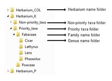
Figure 14.3: Recommended folder structure for storing herbarium images
Annex B. Extended List of Ecogeographic Data Descriptors
The ecogeographic data collection template is based on the template produced by the Millennium Seed Bank Enhancement Project Species Targeting Team (2004–2008), where it was used to capture all information from herbarium labels and subsequently georeference the locality data. The general template from the Botanical Records and Herbarium Management (BRAHMS) rapid data entry system was tailored to follow Royal Botanical Gardens, Kew’s core field standards, and the specific requirements of the project. The format allows the data to be directly used for analysis and mapping. The data collected formed the basis of seed collecting guides produced by Kew and distributed to collecting partners.
In the Adapting Agriculture to Climate Change project (see above), data will be utilized for gap analyses, as well as the production of collection guides. To reflect this extended use, additional fields have been added to the original template. These facilitate the collection of data from a wide range of sources (including public and private digital datasets, herbarium vouchers and genebank datasets) and the management of restrictions on data usage. The modifications were developed collaboratively by the Royal
Botanical Gardens, Kew; the International Centre for Tropical Agriculture (CIAT); and the University of Birmingham. As such, the data types are extensive but it is not necessary to have a complete set to undertake an ecogeographic analysis. However, the more complete the set, the more sophisticated the analysis and the more detailed the prediction and, ultimately, the conservation.
Click here to open a table of the Ecogeographic Data Descriptors.
Comments
- No comments found
Leave your comments
Post comment as a guest